1. The Hybrid Search Score-Fusion Problem: You Can’t Just Add BM25 and Vector Scores
Hybrid search — combining keyword search (full-text search such as BM25) with vector search (embedding similarity search) — has become a standard component of modern search stacks. That’s because the two approaches have complementary weaknesses: vector search is strong on semantic closeness but weak on “exact match on wording” (proper nouns, model numbers), while BM25 is strong on exact matches but weak against vocabulary mismatch (paraphrasing). (This contrast is covered in detail in Chapter 1 of ANN Fundamentals (in Japanese).)
The question is how to merge the two result lists into a single ranking. The naive idea — “just add the two scores” — doesn’t work, for two main reasons. First, the scales are different: BM25 scores have no theoretical upper bound and shift in magnitude depending on query length and IDF (inverse document frequency), while cosine similarity is bounded to \([-1,1]\) (effectively \([0,1]\) for normalized vectors). A naive sum lets whichever score happens to be larger dominate the result almost unilaterally, and because that score distribution shifts from query to query, any fixed pre-normalization coefficient can’t be trusted either. Second, the scores mean different things: a BM25 score measures “how statistically rare the matched terms are,” while cosine similarity measures “an angle in vector space.” These are quantities with different units and different meanings, so adding them together has no mathematical justification to begin with.
One practical solution to this problem is to stop comparing the raw scores altogether and instead fuse the results using only each list’s “rank.” Rank is always a common yardstick — \(1, 2, 3, \dots\) — so it treats the output of any search engine, whether BM25 or vector search, fairly. The formalization of this idea is this article’s subject: Reciprocal Rank Fusion (RRF).
2. Defining RRF and Verifying It by Hand
RRF is a simple scoring formula for fusing multiple rankings, proposed by Cormack, Clarke, and Büttcher in their 2009 SIGIR paper ( Reciprocal Rank Fusion outperforms Condorcet and Individual Rank Learning Methods , SIGIR'09). Given a set of documents \(D\) and a set of rankings \(R\) , the RRF score of a document \(d \in D\) is computed as:
\[ \text{RRF}(d) = \sum_{i \in R} \frac{1}{k + \text{rank}_i(d)} \]Here \(\text{rank}_i(d)\) is the rank (a 1-based integer) of document \(d\) in ranking \(i\) , and \(k\) is a smoothing constant. Sorting documents by this RRF score in descending order gives the final fused ranking.
The paper explains the reasoning behind this formula: “while highly-ranked documents are more important, the importance of lower-ranked documents does not vanish… The constant k mitigates the impact of high rankings by outlier systems.” In other words, unlike an exponentially decaying function, this formula ensures that lower-ranked documents don’t lose all their importance, and the constant \(k\) dampens the effect of any one outlier system pushing a particular document to an unduly high rank.
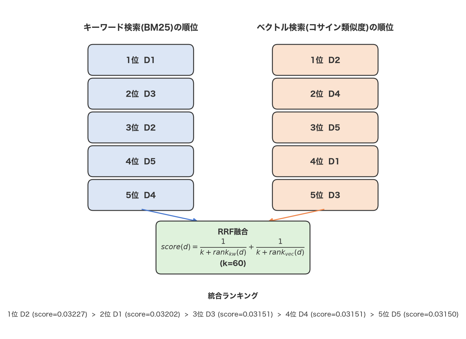
Words alone are hard to internalize, so let’s compute an actual example with \(k=60\) using two rank lists (keyword search and vector search) over five documents, D1 through D5.
| Document | Keyword search rank | Vector search rank | \(\frac{1}{60+\text{rank}_{kw}}\) | \(\frac{1}{60+\text{rank}_{vec}}\) | RRF score |
|---|---|---|---|---|---|
| D1 | 1 | 4 | 0.016393 | 0.015625 | 0.032018 |
| D2 | 3 | 1 | 0.015873 | 0.016393 | 0.032266 |
| D3 | 2 | 5 | 0.016129 | 0.015385 | 0.031514 |
| D4 | 5 | 2 | 0.015385 | 0.016129 | 0.031514 |
| D5 | 4 | 3 | 0.015625 | 0.015873 | 0.031498 |
The fused ranking comes out to D2 (0.032266) > D1 (0.032018) > D3 = D4 (0.031514, an exact tie) > D5 (0.031498). The exact tie between D3 and D4’s RRF scores is no coincidence. D3’s ranks are \((2, 5)\) and D4’s are \((5, 2)\) — the two documents simply have their roles swapped across the two rankings, and \(\frac{1}{k+2}+\frac{1}{k+5}\) equals \(\frac{1}{k+5}+\frac{1}{k+2}\) ; only the order of addition differs. This numerical example confirms directly that RRF cares only about the multiset of ranks a document receives, not which specific ranking produced which rank.
3. Why Rank-Based Fusion Is Robust: Invariance to Score Scale
The biggest reason RRF is favored in practice is that it’s invariant to any monotonic transformation of the underlying scores. Apply any rank-preserving transformation to a ranking’s raw scores — multiplying by a constant, adding a constant, taking a logarithm, applying a sigmoid, or any strictly increasing function — and \(\text{rank}_i(d)\) doesn’t change at all. That means the fused result is unaffected whether a BM25 implementation change scales its scores by 10x, or a swapped embedding model shifts the cosine similarity distribution entirely.
This sets RRF apart not only from naive score addition but also from techniques like min-max normalization that “align scores before combining them.” Min-max normalization requires recomputing the minimum and maximum for every query, and a single outlier can distort the entire post-normalization distribution. Because RRF never looks at the score values in the first place, this kind of calibration work becomes unnecessary in principle. The paper itself points to the implementation benefits: “RRF… combines ranks without regard to the arbitrary scores returned by particular ranking methods… ranks may be computed and summed one system at a time, avoiding the necessity of keeping all rankings in memory.” As long as you know the ranks, you can accumulate the score system by system, without ever having to hold every ranking in memory simultaneously. The experiments below quantify how much this “score-scale invariance” actually matters in practice.
4. Experiment: Fusing Two Imperfect Rankers
Setup
We build a synthetic dataset of \(N=1000\)
documents, of which 50 are randomly designated as “true relevant documents.” These 50 are further split into two groups of 25: one where a “keyword-leaning ranker” excels, and one where a “semantic-leaning ranker” excels. Each ranker’s score is generated as follows (seeded with NumPy’s default_rng):
- Documents in its strong group: score drawn from a normal distribution with mean \(\mu_{hi}=2.0\) , std \(\sigma=1.0\) (a strong positive signal)
- Documents in its weak group: mean \(\mu_{lo}=1.0\) , same \(\sigma=1.0\) (a weak but reliably positive signal)
- The 950 irrelevant documents: mean \(0\) , same \(\sigma=1.0\) (no signal)
Keyword-leaning ranker A uses \(\mu_{hi}\) for the “keyword group” and \(\mu_{lo}\) for the “semantic group”; semantic-leaning ranker B does the opposite (\(\mu_{hi}\) for the semantic group, \(\mu_{lo}\) for the keyword group). In other words, neither ranker is completely blind to the half of relevant documents it isn’t good at — it just gets a weaker signal there. This is a simplified model of the real asymmetry that motivates hybrid search: BM25 can partially, but not fully, catch paraphrased content, and vector search can somewhat, but not decisively, catch rare exact-match terms.
For evaluation, letting \(\text{rel}_i\) be the relevance (1 = relevant, 0 = irrelevant) of the document at rank \(i\) , we use the following nDCG (normalized Discounted Cumulative Gain):
\[ \text{DCG@k} = \sum_{i=1}^{k} \frac{\text{rel}_i}{\log_2(i+1)}, \qquad \text{nDCG@k} = \frac{\text{DCG@k}}{\text{IDCG@k}} \]\(\text{IDCG@k}\) is the DCG@k under the ideal ordering (relevant documents sorted first), which normalizes nDCG to \([0,1]\) . recall@k is “the number of relevant documents in the top k, divided by the total number of relevant documents” (with 50 relevant documents in this setup, the theoretical ceiling for recall@10 is \(10/50=0.20\) ).
Implementation (excerpt)
import numpy as np

def ndcg_at_k(rel_in_rank_order, k):
    rel = np.asarray(rel_in_rank_order[:k], dtype=float)
    dcg = np.sum(rel / np.log2(np.arange(2, len(rel) + 2)))
    ideal = np.sort(rel_in_rank_order)[::-1]
    idcg = np.sum(ideal[:k] / np.log2(np.arange(2, len(ideal[:k]) + 2)))
    return dcg / idcg if idcg > 0 else 0.0

def rrf_fuse(orders, k=60, n_docs=1000):
    """orders: array of document indices per ranking (index 0 = rank 1)"""
    total = np.zeros(n_docs)
    for order in orders:
        rank = np.empty(n_docs, dtype=int)
        rank[order] = np.arange(1, n_docs + 1)
        total += 1.0 / (k + rank)
    return np.argsort(-total)  # fused rank order
Measured results
Averaged over 300 seeded trials (standard deviation also shown):
| Metric | Keyword-leaning ranker alone | Semantic-leaning ranker alone | RRF fusion (k=60) |
|---|---|---|---|
| nDCG@10 | 0.7346 ± 0.0914 | 0.7260 ± 0.1027 | 0.8807 ± 0.0983 |
| recall@10 | 0.1365 ± 0.0278 | 0.1355 ± 0.0290 | 0.1713 ± 0.0224 |
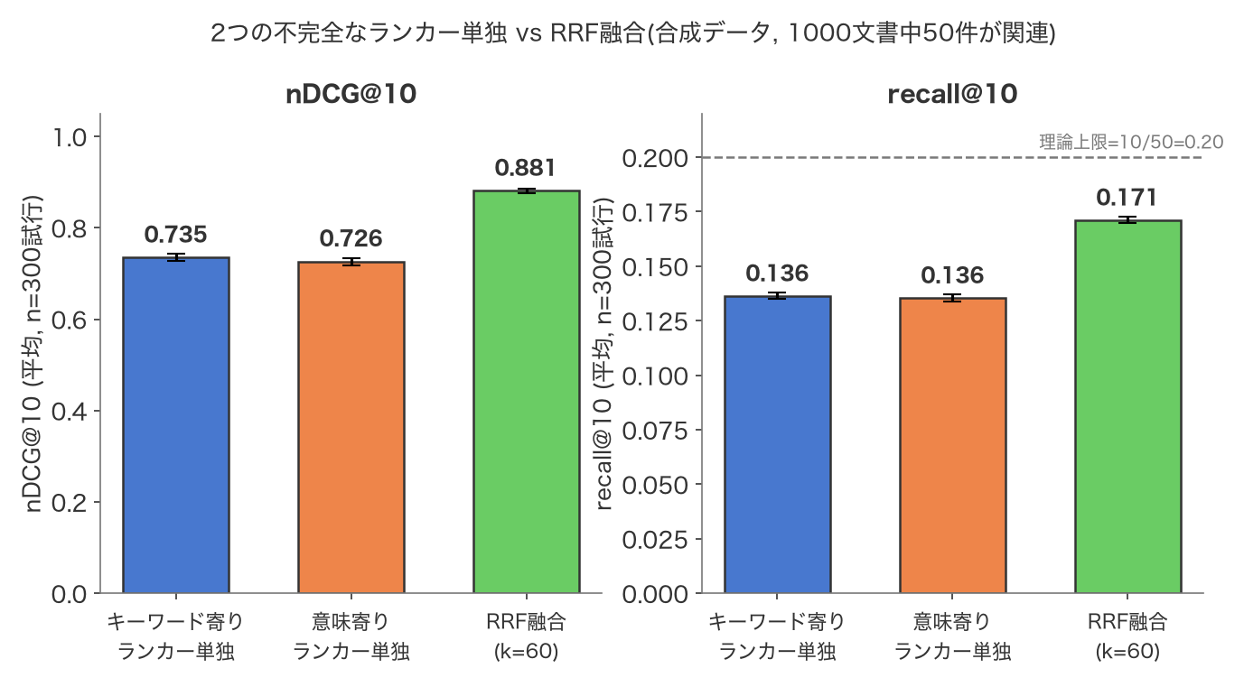
RRF fusion beat the single rankers by 14–15 points on nDCG@10 and by around 3.5 points on recall@10. Against the recall@10 ceiling of 0.20, the single rankers only reach 0.136 (about 68% of the ceiling), while RRF fusion reaches 0.171 (about 85% of the ceiling). This is because every relevant document receives a positive signal (strong or weak) from at least one of the two rankers, and the rank-based sum accumulates that “weak consensus across multiple systems” to surface it. Neither single ranker can reliably promote the half of relevant documents it’s weak on, but RRF fusion properly picks up documents that either ranker strongly supports. This is exactly the motivation for combining BM25 with vector search in real hybrid search, and even in this simplified synthetic setting, the same effect is confirmed quantitatively.
5. Experiment: Sensitivity to k, and Where k=60 Comes From
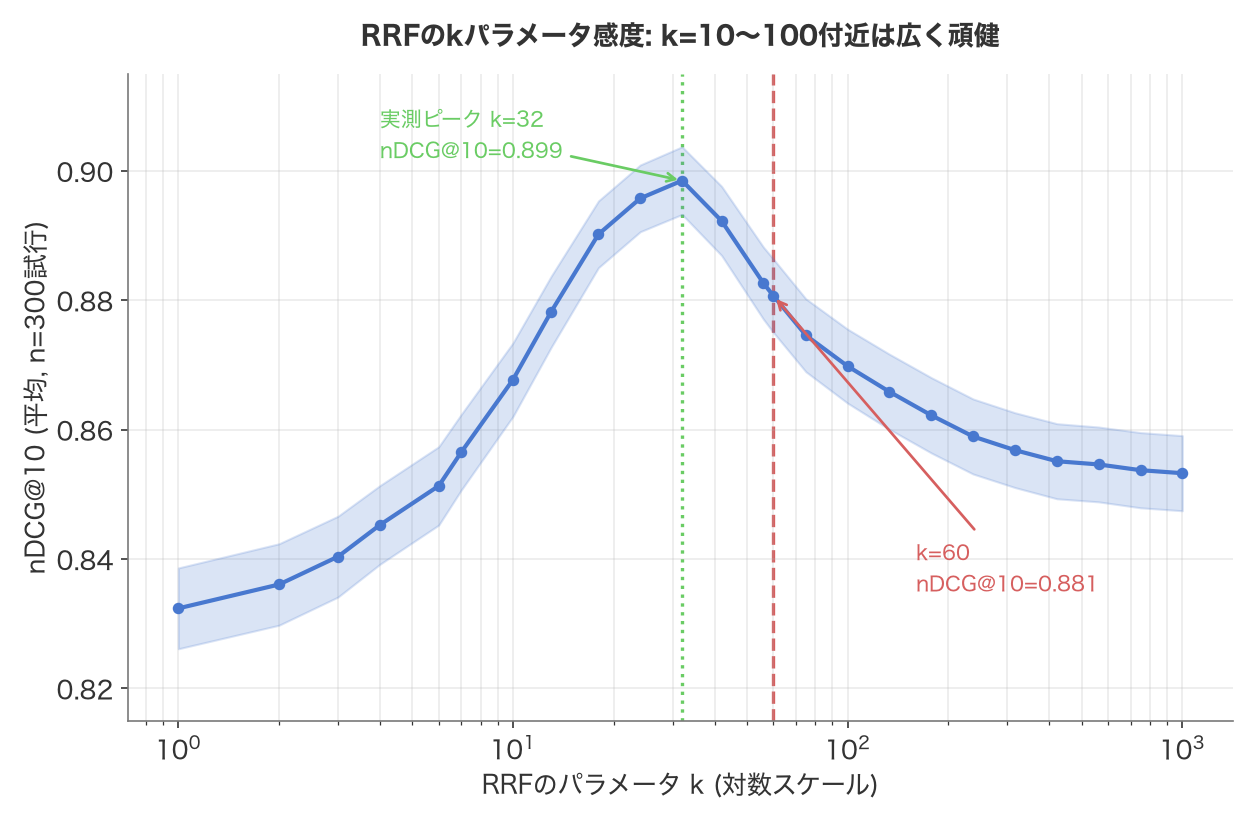
Using the same 300 trials and the same score-generation process as Experiment 4, we swept RRF’s only parameter, \(k\) , from \(k=1\) to \(k=1000\) on a log scale and measured how nDCG@10 changed.
| \(k\) | 1 | 10 | 32 (measured peak) | 60 | 100 | 316 | 1000 |
|---|---|---|---|---|---|---|---|
| nDCG@10 | 0.832 | 0.868 | 0.899 | 0.881 | 0.870 | 0.857 | 0.853 |
The measured peak is at \(k=32\) (nDCG@10=0.899), but across \(k=10\) to \(k=100\) , nDCG@10 stays between 0.868 and 0.899 — a very gentle hill. Even at the extreme of \(k=1\) it’s 0.832, and at \(k=1000\) it’s 0.853 — dropping less than 10 points from the peak in either direction. In other words, shifting \(k\) around doesn’t cause a catastrophic performance drop; RRF is broadly robust to this parameter, as confirmed quantitatively on this synthetic data.
This robustness was itself discovered first by Cormack, Clarke, and Büttcher’s original paper. Table 1 of the paper shows a pilot experiment fusing the results of 30 model systems on TREC topics 351–400, sweeping \(k\) from 0 to 500 and measuring MAP (Mean Average Precision):
| \(k\) | 0 | 10 | 20 | 30 | 40 | 50 | 60 | 70 | 80 | 90 | 100 | 500 |
|---|---|---|---|---|---|---|---|---|---|---|---|---|
| MAP | .2072 | .2123 | .2134 | .2139 | .2138 | .2144 | .2145 | .2146 | .2147 | .2145 | .2142 | .2098 |
The paper states plainly: “The results of the first, shown in table 1, indicated that k = 60 was near-optimal, but that the choice was not critical.”
In other words, there is nothing mathematically special about the value \(k=60\) itself — it was simply a near-optimal value found in the authors’ pilot experiment, which they then “fixed… and not altered during subsequent validation” (the paper’s own phrasing: “where k = 60 was fixed during a pilot investigation and not altered during subsequent validation”). The fact that Milvus, OpenSearch, and Elasticsearch all adopt \(k=60\) (or an equivalent default) as their default is best understood as an industry convention that has held up as “good enough” across nearly two decades of follow-up validation since this paper, rather than any inherent mathematical necessity.
The paper also shows that RRF consistently outperforms Condorcet Fuse and CombMNZ (another fusion method combining scores and ranks). In an experiment fusing the actual submitted rankings from participants across four TREC tasks — TREC Robust, TREC 3, TREC 5, and TREC 9 (Table 2) — RRF’s MAP beat Condorcet Fuse in all four cases and CombMNZ in 3 of 4 cases. In the final experiment on the LETOR 3 dataset (583,850 query-document pairs, Table 3), RRF beat every individual method, including learning-to-rank methods such as RankSVM, RankBoost, AdaRank-MAP, and ListNet, at \(p<.003\) (a margin of 0.02 in MAP, about 4%, over the best individual method).
6. When to Use Min-Max Normalization-Based Fusion Instead
To check how much RRF’s “score-scale invariance” actually matters in practice, we ran a fusion experiment on the same two rankers from Experiment 4, but deliberately gave them an extreme scale mismatch. Ranker A’s scores are left as-is; ranker B’s scores are put through the monotonic transformation \(\text{score}_B' = 400 \times \text{score}_B + 5000\) (modeling A as a small-magnitude BM25-like score and B as a large-magnitude inner-product-like score — since it’s a monotonic transformation, it shouldn’t affect the fused result in principle). Under this condition we compared (1) naive raw score addition, (2) addition after per-query min-max normalization, and (3) RRF.
\[ \text{minmax}(x) = \frac{x - \min(x)}{\max(x) - \min(x)} \]| Metric | Ranker A alone | Ranker B alone | Raw score sum | Min-max normalized sum | RRF (k=60) |
|---|---|---|---|---|---|
| nDCG@10 | 0.7332 | 0.7320 | 0.7335 | 0.9046 | 0.8858 |
| recall@10 | 0.1370 | 0.1356 | 0.1359 | 0.1753 | 0.1719 |
The naive raw score sum gives an nDCG@10 of 0.7335 — essentially identical to ranker B alone (0.7320). In other words, the larger-scale ranker B ends up dominating the fused result almost unilaterally, and ranker A’s information is effectively buried in noise and ignored. This is the measured reproduction of the “naive addition doesn’t work” claim from the opening section.
Min-max normalization before summing, on the other hand, recovers an nDCG@10 of 0.9046 — in this experiment, slightly ahead of RRF (0.8858). Min-max normalization can preserve “magnitude information” (e.g., the difference between similarities of 0.95 and 0.60) while fusing, which can work in RRF’s favor when that difference carries real meaning. In practice, OpenSearch offers exactly this kind of score-based fusion via its normalization-processor (min-max or L2 normalization combined with arithmetic/geometric/harmonic mean), officially supported alongside RRF.
That said, min-max normalization has to recompute min/max on every query, and a single outlier can distort the normalized distribution as a whole. Because RRF never looks at the score values at all, this kind of calibration is unnecessary in principle, making it structurally robust to swapped embedding models or shifting score distributions. As a rule of thumb: use min-max normalization when scores across lists are calibrated with the same semantics and the “size of the difference” itself carries value; prefer RRF’s robustness when score semantics or distributions can vary wildly across lists or queries. The two aren’t mutually exclusive — OpenSearch’s design of supporting both within its search pipeline, letting you switch based on the use case, is a sensible approach in practice.
7. Implementation: Using RRF in Milvus, OpenSearch, and Elasticsearch
Milvus: RRFRanker
Milvus supports RRF fusion via its hybrid_search() API and RRFRanker class. The default \(k\)
is 60, with a valid range of \((0, 16384)\)
(
Milvus documentation: RRF Ranker
). Milvus’s internal architecture — Query Nodes, segments, consistency levels, and more — is covered in
Milvus Internals
(in Japanese).
from pymilvus import MilvusClient, AnnSearchRequest, RRFRanker

client = MilvusClient(uri="http://localhost:19530")

# BM25 full-text search (sparse_vector field)
req_bm25 = AnnSearchRequest(
    data=["how does vector search work"],
    anns_field="sparse_vector",
    param={"metric_type": "BM25"},
    limit=20,
)
# Dense embedding search (dense_vector field)
req_dense = AnnSearchRequest(
    data=[query_embedding],
    anns_field="dense_vector",
    param={"metric_type": "COSINE"},
    limit=20,
)

ranker = RRFRanker(k=60)  # default k=60, range (0, 16384)

results = client.hybrid_search(
    collection_name="docs",
    reqs=[req_bm25, req_dense],
    ranker=ranker,
    limit=10,
)
OpenSearch: score-ranker-processor (RRF) and normalization-processor
OpenSearch 2.19 added a score-ranker-processor to the Neural Search plugin, supporting RRF as an rrf combination technique (
Introducing reciprocal rank fusion for hybrid search - OpenSearch
,
Score ranker - OpenSearch Documentation
). The default rank_constant is 60 (minimum 1). It’s defined as a search pipeline and specified via a query parameter on the search request. OpenSearch’s k-NN search internals are covered in
OpenSearch k-NN Internals
(in Japanese).
PUT /_search/pipeline/rrf-pipeline
{
  "description": "Fusion pipeline for RRF-based hybrid search",
  "phase_results_processors": [
    {
      "score-ranker-processor": {
        "combination": {
          "technique": "rrf",
          "rank_constant": 60
        }
      }
    }
  ]
}
POST my_index/_search?search_pipeline=rrf-pipeline
As mentioned in the previous section, OpenSearch also separately provides a score-based fusion technique, normalization-processor (min-max or L2 normalization), which can be used instead of RRF depending on requirements (
Normalization processor - OpenSearch Documentation
).
Elasticsearch: the rrf retriever
Elasticsearch provides an rrf retriever that fuses results from multiple child retrievers (a standard query, a knn query, and so on) (
Reciprocal rank fusion - Elasticsearch Reference
). The parameter is named rank_constant (default 60, minimum 1), and you also specify rank_window_size, which controls how many results per retriever are considered for fusion.
{
  "retriever": {
    "rrf": {
      "retrievers": [
        {
          "standard": {
            "query": { "match": { "text": "vector search" } }
          }
        },
        {
          "knn": {
            "field": "vector",
            "query_vector": [0.12, 0.34, -0.05],
            "k": 50,
            "num_candidates": 100
          }
        }
      ],
      "rank_window_size": 50,
      "rank_constant": 60
    }
  }
}
All three systems use the exact same formula as the original RRF paper, and it’s notable that both the parameter naming (k / rank_constant) and the default value (60) have effectively converged into an industry standard.
Summary
- RRF is the simple formula \(\text{RRF}(d) = \sum_{i} \frac{1}{k+\text{rank}_i(d)}\) , fusing multiple search results using only their “rank.” Because it never looks at raw score values, it can fairly fuse scores with different scales and different meanings — like BM25 and vector search — without any calibration.
- In experiments on synthetic data, RRF fusion of two imperfect rankers (keyword-leaning and semantic-leaning) clearly beat either ranker alone on both nDCG@10 and recall@10 (+0.146 to +0.155 on nDCG@10; recall@10 rose from 68% to 85% of its theoretical ceiling).
- The \(k\) -sweep experiment showed nDCG@10 staying at a gently high level across the wide range \(k=10\) to \(100\) , and the original paper itself states that “k=60 was near-optimal, but the choice was not critical.”
- Under extreme score-scale mismatch, naive addition failed (dominated by the larger-scale ranker), while both min-max normalization and RRF recovered good results. Choosing between them is a practical, use-case-dependent decision.
- Milvus, OpenSearch, and Elasticsearch all officially support RRF implementations with a default of \(k\)
(or
rank_constant) = 60.
Frequently Asked Questions (FAQ)
Q. What value should I use for k?
Both the original paper’s pilot experiment (Table 1) and this article’s own experiments show that within the range \(k=10\) to \(100\) , nDCG@10 changes only gently, with no catastrophic degradation. Start with the default of 60 used by Milvus, OpenSearch, and Elasticsearch alike, measure your own evaluation metrics (nDCG, recall) on your dataset, and lightly sweep the 10-to-100 range if needed. There’s no mathematical necessity behind the number 60 itself — think of it as a well-established default that has held up across nearly two decades of follow-up validation.
Q. Should I use RRF or score normalization (min-max, etc.)?
If your search engines’ scores are calibrated with the same semantics and the “size of the difference” itself carries meaning (e.g., you trust that a similarity of 0.9 versus 0.5 means something), score-based fusion methods like min-max normalization can make use of more information. If you’re combining multiple engines or models, or if score distributions swing widely from query to query, RRF’s scale-independent robustness has the edge. A practical landing point, as OpenSearch does, is to offer both within your search pipeline and switch based on requirements.
Q. Can I fuse results from three or more systems?
Yes. RRF’s formula, \(\sum_{i \in R} \frac{1}{k+\text{rank}_i(d)}\)
, isn’t limited to \(|R|=2\)
— you simply sum over however many rankings you have. For example, fusing four systems — BM25, dense vector search, sparse vector search (e.g., SPLADE), and a metadata-based business-rule score — just means summing four terms. If you want to weight some systems more heavily than others, you can use a weighted extension (weighted RRF), such as Milvus’s WeightedRanker, which applies a weight to each term.
Related Articles
- ANN Fundamentals: How HNSW, IVF, PQ, and DiskANN Work (in Japanese) - Covers, down to the level of formulas, why BM25 and vector search complement each other and how recall@k is defined and measured.
- What Is RAG? A Thorough Guide to How Retrieval-Augmented Generation Works and How to Build It, from Vector Search Fundamentals - Explains where RRF fits within RAG’s retrieval-quality improvement pipeline, alongside cross-encoder reranking and query transformation.
- Milvus Internals
(in Japanese) - Covers the distributed architecture underlying
hybrid_search()and RRFRanker. - OpenSearch k-NN Internals
(in Japanese) - Covers the internal implementation of the search pipeline that runs
score-ranker-processorandnormalization-processor.
Classic books covering other fields are collected in 10 Technical Books Every Engineer Should Read .
References
Paper
- Cormack, G. V., Clarke, C. L. A., and Büttcher, S., “Reciprocal Rank Fusion outperforms Condorcet and Individual Rank Learning Methods”, SIGIR'09 - The original paper proposing RRF (hosted by the authors). ACM Digital Library