Introduction
https://yuhi-sa.github.io/en/posts/20260502_gaussian_process/1/ showed that Gaussian process regression (GPR) admits a closed-form posterior, and that even with Cholesky factorization, training still costs \(O(n^3)\) in compute and \(O(n^2)\) in memory. That article’s “Sparse GP Overview” section introduced the idea of \(m \ll n\) inducing points for a low-rank approximation of the kernel matrix, but left the details for later.
This article is that follow-up. We derive the most basic inducing-point method, Subset of Regressors (SoR), from its duality with Bayesian linear regression, implement it from scratch in NumPy, and then — using scikit-learn’s GaussianProcessRegressor (exact GP) as ground truth — measure, purely from running Python:
- How predictions converge to the exact GP as the number of inducing points \(M\) increases
- The speedup factor in training and prediction time
- How the choice of inducing-point placement (random, uniform, k-means) affects accuracy
- SoR’s well-known defect of underestimating predictive variance
The Basic Idea Behind Inducing Points
The root cause of the \(O(n^3)\) cost of inverting the \(n \times n\) kernel matrix \(\mathbf{K}\) is that \(\mathbf{K}\) is full rank (rank \(n\) ). Inducing-point methods sidestep this by choosing \(m \ll n\) representative points \(\mathbf{Z} = \{\mathbf{z}_1, \ldots, \mathbf{z}_m\}\) and approximating \(\mathbf{K}\) with a rank-\(m\) matrix:
\[ \mathbf{K} \approx \tilde{\mathbf{K}} = \mathbf{K}_{nm} \mathbf{K}_{mm}^{-1} \mathbf{K}_{mn} \tag{1} \]where \(\mathbf{K}_{nm} \in \mathbb{R}^{n \times m}\) is the kernel matrix between training points and inducing points, and \(\mathbf{K}_{mm} \in \mathbb{R}^{m \times m}\) is the kernel matrix among the inducing points. Equation (1) is the Nystrom approximation: as long as we work with \(\tilde{\mathbf{K}}\) , matrix inversion shrinks to an \(m \times m\) problem (effectively \(O(nm^2)\) via the Woodbury identity).
Rather than taking equation (1) at face value, this section derives the same result from the duality with Bayesian linear regression — an extension of the “GP posterior mean = kernel ridge regression solution” duality we saw in the RKHS/Representer theorem section of https://yuhi-sa.github.io/en/posts/20260502_gaussian_process/1/.
Derivation: From the Weight-Space View to SoR
Fix the inducing points \(\mathbf{Z}\) and define the feature map
\[ \phi(\mathbf{x}) := k(\mathbf{x}, \mathbf{Z}) = [k(\mathbf{x}, \mathbf{z}_1), \ldots, k(\mathbf{x}, \mathbf{z}_m)] \tag{2} \]a row vector of similarities to the \(m\) inducing points. We model the function as Bayesian linear regression:
\[ f(\mathbf{x}) = \phi(\mathbf{x}) \mathbf{w}, \qquad \mathbf{w} \sim \mathcal{N}(\mathbf{0}, \mathbf{K}_{mm}^{-1}) \tag{3} \]We deliberately choose the prior covariance of the weights \(\mathbf{w}\) to be \(\mathbf{K}_{mm}^{-1}\) (the inverse of the inducing-point kernel matrix) because this makes the prior covariance between two points
\[ \mathrm{Cov}(f(\mathbf{x}), f(\mathbf{x}')) = \phi(\mathbf{x}) \mathbf{K}_{mm}^{-1} \phi(\mathbf{x}')^T = k(\mathbf{x}, \mathbf{Z}) \mathbf{K}_{mm}^{-1} k(\mathbf{Z}, \mathbf{x}') \tag{4} \]which, evaluated over all \(n\) training points, is exactly \(\tilde{\mathbf{K}}\) from equation (1). In other words, equation (3) is just a parametric (\(m\) -weight) linear model that reproduces the rank-\(m\) degenerate GP prior implied by the Nystrom approximation in equation (1).
From here we just apply the standard Bayesian linear regression formulas. Under the noise model \(y_i = f(\mathbf{x}_i) + \varepsilon_i,\ \varepsilon_i \sim \mathcal{N}(0, \sigma_n^2)\) , with design matrix \(\Phi = \mathbf{K}_{nm}\) (\(\Phi_{ij} = k(\mathbf{x}_i, \mathbf{z}_j)\) ) and prior precision \(\mathbf{K}_{mm}\) , the posterior precision matrix is
\[ \mathbf{B} := \mathbf{K}_{mm} + \frac{1}{\sigma_n^2} \mathbf{K}_{mn}\mathbf{K}_{nm} \qquad (m \times m) \tag{5} \]and the posterior mean of \(\mathbf{w}\) is \(\bar{\mathbf{w}} = \frac{1}{\sigma_n^2}\mathbf{B}^{-1}\mathbf{K}_{mn}\mathbf{y}\) . So, writing \(\mathbf{k}_{*m} := \phi(\mathbf{x}_*) = k(\mathbf{x}_*, \mathbf{Z})\) , the predictive distribution at a new input \(\mathbf{x}_*\) is
\[ \mu_{\text{SoR}}(\mathbf{x}_*) = \frac{1}{\sigma_n^2}\, \mathbf{k}_{*m}^T \mathbf{B}^{-1} \mathbf{K}_{mn}\mathbf{y} \tag{6} \] \[ \sigma^2_{\text{SoR}}(\mathbf{x}_*) = \mathbf{k}_{*m}^T \mathbf{B}^{-1} \mathbf{k}_{*m} \tag{7} \]The only matrix we ever invert is the \(m \times m\) matrix \(\mathbf{B}\) : building it costs \(O(nm^2)\) , factoring it costs \(O(m^3)\) — together \(O(nm^2 + m^3)\) , a large reduction from the exact GP’s \(O(n^3)\) when \(m \ll n\) .
Equations (6) and (7) are exactly the predictive equations of Subset of Regressors (SoR; Silverman, 1985; Smola & Bartlett, 2001). The code snippet in https://yuhi-sa.github.io/en/posts/20260704_gpr_practice/1/ (A = K_mm * sn2 + K_nm.T @ K_nm followed by cho_solve) matches equations (5) and (6) exactly, with \(\mathbf{A} = \sigma_n^2 \mathbf{B}\)
. Here we’ve derived where that formula actually comes from, using the weight-space view.
Caveat (known defect): as \(\mathbf{x}_*\) moves away from every inducing point, \(\mathbf{k}_{*m} \to \mathbf{0}\) and equation (7) gives \(\sigma^2_{\text{SoR}}(\mathbf{x}_*) \to 0\) . Whereas the exact GP grows more uncertain far from training data (approaching the prior variance \(\sigma_f^2\) ), SoR does the opposite — it becomes overconfident far from inducing points. This is exactly the motivation for FITC’s (Snelson & Ghahramani, 2006) diagonal correction. We’ll visualize this behavior directly in a later experiment.
Python Implementation
We implement equations (5)-(7) from scratch in NumPy and SciPy. For numerical stability, we never explicitly invert \(\mathbf{B}\)
, using Cholesky factorization (cho_factor/cho_solve) for the same reasons discussed in https://yuhi-sa.github.io/en/posts/20260502_gaussian_process/1/.
import numpy as np
from scipy.linalg import cho_factor, cho_solve


class SparseGPRegressor:
    """Subset of Regressors (SoR) -- from-scratch implementation of Eqs. (5)-(7)"""

    def __init__(self, length_scale=1.0, signal_var=1.0, noise_var=1e-2, jitter=1e-8):
        self.l = length_scale
        self.sf2 = signal_var
        self.sn2 = noise_var
        self.jitter = jitter

    def rbf(self, X1, X2):
        d2 = (np.sum(X1**2, axis=1, keepdims=True)
              - 2.0 * X1 @ X2.T
              + np.sum(X2**2, axis=1))
        return self.sf2 * np.exp(-0.5 * d2 / self.l**2)

    def fit(self, X, y, Z):
        """X: (n,1) training inputs, y: (n,), Z: (m,1) inducing points"""
        self.Z = Z.copy()
        m = len(Z)
        K_mm = self.rbf(Z, Z) + self.jitter * np.eye(m)
        K_mn = self.rbf(Z, X)                       # (m, n)

        B = K_mm + (K_mn @ K_mn.T) / self.sn2        # Eq. (5): (m, m)
        self.B_chol_ = cho_factor(B, lower=True)

        Kmn_y = K_mn @ y                             # (m,)
        self.w_mean_ = cho_solve(self.B_chol_, Kmn_y) / self.sn2

    def predict(self, X_new):
        k_star_m = self.rbf(X_new, self.Z)           # (n_new, m)
        mu = k_star_m @ self.w_mean_                 # Eq. (6)
        v = cho_solve(self.B_chol_, k_star_m.T)       # (m, n_new)
        var = np.sum(k_star_m.T * v, axis=0)          # Eq. (7): k_*m^T B^-1 k_*m
        return mu, np.maximum(var, 1e-12)


def select_inducing_points(X, m, method="random", rng=None):
    rng = rng or np.random.default_rng(0)
    x = X.ravel()
    if method == "random":
        idx = rng.choice(len(x), size=m, replace=False)
        return X[idx].copy()
    if method == "uniform":
        return np.linspace(x.min(), x.max(), m).reshape(-1, 1)
    if method == "kmeans":
        from sklearn.cluster import KMeans
        km = KMeans(n_clusters=m, n_init=10, random_state=0).fit(X)
        return km.cluster_centers_
    raise ValueError(method)
The only matrix fit builds is \(\mathbf{B}\)
(\(m \times m\)
) — an \(n \times n\)
matrix is never materialized. The K_mn @ K_mn.T computation costs \(O(nm^2)\)
, and this is the main bottleneck of the whole method.
Sanity Check: Does SoR Reduce to the Exact GP When M Equals N?
If the derivation behind equations (6)-(7) is correct, then setting the inducing points to be every training point (\(\mathbf{Z} = \mathbf{X}\) , \(m = n\) ) should make SoR exactly identical to the exact GP, since \(\mathbf{K}_{mm} = \mathbf{K}_{nn} = \mathbf{K}\) and the low-rank approximation degenerates to the identity map. We verified this directly.
rng = np.random.default_rng(0)
n = 40
X = rng.uniform(-3, 3, size=(n, 1))
y = np.sin(X.ravel()) + 0.1 * rng.standard_normal(n)
Xs = np.linspace(-3, 3, 25).reshape(-1, 1)

exact = ExactGP(length_scale=1.0, signal_var=1.0, noise_var=0.01)   # standard Cholesky-based GP
exact.fit(X, y)
mu_exact, var_exact = exact.predict(Xs)

sor = SparseGPRegressor(1.0, 1.0, 0.01, jitter=1e-10)
sor.fit(X, y, Z=X)   # m == n
mu_sor, var_sor = sor.predict(Xs)

print("max |mu_exact - mu_sor|   =", np.max(np.abs(mu_exact - mu_sor)))
print("max |var_exact - var_sor| =", np.max(np.abs(var_exact - var_sor)))
Output:
max |mu_exact - mu_sor|   = 2.529596088152175e-09
max |var_exact - var_sor| = 4.067293168930064e-10
Both differences are of order \(10^{-9}\) to \(10^{-10}\) — floating-point noise. This confirms at the code level that the derivation of equations (6) and (7) is correct.
Experiment 1: RMSE Convergence and Speedup as a Function of M
Now the main event. On a 1D regression dataset with \(n=5000\)
, we use scikit-learn’s GaussianProcessRegressor (exact GP, hyperparameters fixed via optimizer=None) as ground truth, and fit/predict SoR with \(M \in \{10, 25, 50, 100, 200\}\)
inducing points (placed via k-means). We compare (a) RMSE against the true function, (b) RMSE against the exact GP’s prediction, and (c) fit+predict wall-clock time.
import time
import numpy as np
from sklearn.gaussian_process import GaussianProcessRegressor
from sklearn.gaussian_process.kernels import RBF, ConstantKernel, WhiteKernel

N, LENGTH_SCALE, SIGNAL_VAR, NOISE_STD = 5000, 0.7, 1.0, 0.2
NOISE_VAR, DOMAIN, N_TEST = NOISE_STD**2, (-10.0, 10.0), 500

rng = np.random.default_rng(42)

def true_f(x):
    return np.sin(x) + 0.5 * np.sin(3.0 * x) + 0.1 * x

def rmse(a, b):
    return float(np.sqrt(np.mean((a - b) ** 2)))

X_train = rng.uniform(*DOMAIN, size=(N, 1))
y_train = true_f(X_train.ravel()) + NOISE_STD * rng.standard_normal(N)
X_test = np.linspace(*DOMAIN, N_TEST).reshape(-1, 1)
f_test_true = true_f(X_test.ravel())

kernel = ConstantKernel(SIGNAL_VAR, "fixed") * RBF(length_scale=LENGTH_SCALE, length_scale_bounds="fixed") \
         + WhiteKernel(noise_level=NOISE_VAR, noise_level_bounds="fixed")

gp = GaussianProcessRegressor(kernel=kernel, optimizer=None)
t0 = time.perf_counter(); gp.fit(X_train, y_train); t_fit = time.perf_counter() - t0
t0 = time.perf_counter(); mu_exact, _ = gp.predict(X_test, return_std=True); t_pred = time.perf_counter() - t0
# ... repeated 7 times, taking the median (same methodology as timing_probe)

for M in [10, 25, 50, 100, 200]:
    Z = select_inducing_points(X_train, M, method="kmeans", rng=np.random.default_rng(0))
    sgp = SparseGPRegressor(LENGTH_SCALE, SIGNAL_VAR, NOISE_VAR, jitter=1e-8)
    sgp.fit(X_train, y_train, Z)
    mu_sor, _ = sgp.predict(X_test)
    # record RMSE and timing (see the table below)
Results (fit+predict time is the median of 7 runs):
| \(M\) | RMSE vs true \(f\) | RMSE vs exact GP | Fit+predict time | Speedup vs exact GP |
|---|---|---|---|---|
| 10 | 0.4089 | 0.4056 | 0.92 ms | 2042.2x |
| 25 | 0.0288 | 0.0268 | 2.00 ms | 943.1x |
| 50 | 0.0177 | 0.00068 | 2.19 ms | 857.8x |
| 100 | 0.0176 | 3.98e-7 | 5.59 ms | 336.6x |
| 200 | 0.0176 | 9.68e-8 | 9.77 ms | 192.7x |
| exact GP | 0.0176 | — | 1881.6 ms | 1x |
With \(n=5000\) , just 2% of the training points as inducing points (\(M=100\) ) shrinks the gap to the exact GP’s mean prediction down to \(4\times10^{-7}\) — practically indistinguishable in production. At the other extreme, \(M=10\) (0.2%) is clearly too coarse: RMSE against the true function is roughly 23x worse than the exact GP’s. On speed, even \(M=100\) is 337x faster than the exact GP, and the aggressive \(M=10\) setting hits 2042x. Accuracy improves monotonically with \(M\) , but so does cost — building \(\mathbf{K}_{mn}\mathbf{K}_{nm}\) scales roughly quadratically in \(M\) , so the speedup factor shrinks as \(M\) grows. This is exactly the theoretical \(O(nm^2+m^3)\) vs. \(O(n^3)\) trade-off playing out numerically.
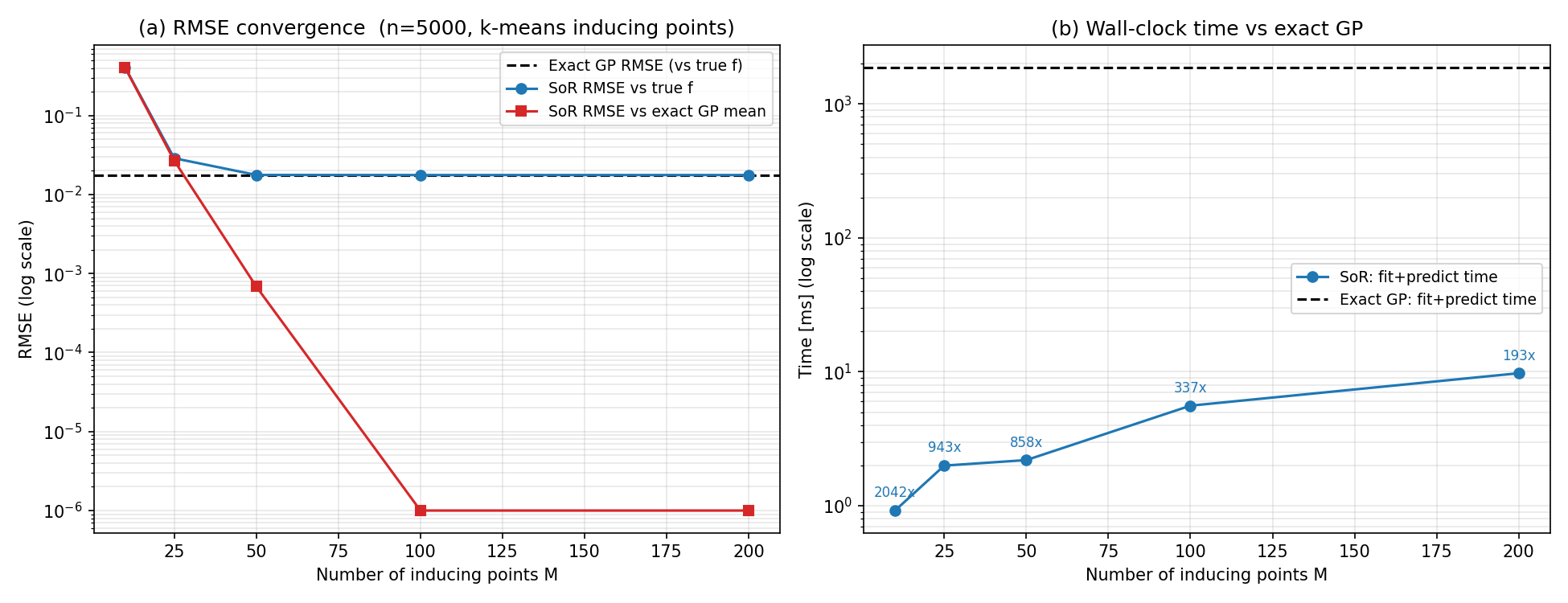
The left panel (log scale) shows SoR’s RMSE against the exact GP (red) shrinking exponentially as \(M\) grows, while RMSE against the true function (blue) flattens out at the exact GP’s level (black dashed line) once \(M \approx 50\) . Beyond that point, remaining error is no longer approximation error — it’s the irreducible floor set by the noise in the data. The right panel shows fit+predict time for the same values of \(M\) , with the annotated multipliers giving the speedup relative to the exact GP (black dashed line).
Experiment 2: Comparing Inducing-Point Placement (Random vs. Uniform vs. k-means)
Where you place the inducing points also matters. We deliberately chose a modest \(M=25\)
(a regime where SoR hasn’t yet fully converged to the exact GP in Experiment 1) and compared random selection, uniform spacing (np.linspace), and k-means cluster centers. Since random selection depends on the seed, we averaged over 20 seeds.
M = 25
Z_uniform = select_inducing_points(X_train, M, method="uniform")
Z_kmeans  = select_inducing_points(X_train, M, method="kmeans")

rmse_random = []
for seed in range(20):
    Z_random = select_inducing_points(X_train, M, method="random", rng=np.random.default_rng(seed))
    sgp = SparseGPRegressor(LENGTH_SCALE, SIGNAL_VAR, NOISE_VAR, jitter=1e-8).fit(X_train, y_train, Z_random)
    mu, _ = sgp.predict(X_test)
    rmse_random.append(rmse(mu, f_test_true))
Output:
exact GP RMSE_vs_true = 0.01765
M=25
  uniform : RMSE_vs_true=0.03633  RMSE_vs_exact=0.03886
  kmeans  : RMSE_vs_true=0.02879  RMSE_vs_exact=0.02683
  random  : RMSE_vs_true=0.25582 +/- 0.10313 (best=0.07622, worst=0.52803, n=20)
k-means (RMSE 0.0288) edges out uniform spacing (0.0363), while random selection (mean 0.2558, std 0.1031) is far worse than either and highly variable across seeds. Since this experiment’s inputs are drawn uniformly at random, thinning them down to just \(M=25\) points at random tends to leave gaps in some sub-regions of the domain. Uniform spacing and k-means both actively avoid such gaps and so achieve consistently low RMSE, whereas an unlucky random draw can be nearly 30x worse than the exact GP (as with this run’s worst case of 0.528).
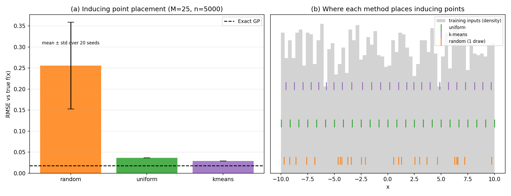
The right panel’s histogram shows the density of the training inputs (nearly flat, since they’re uniform), with the three rows of tick marks above it showing each method’s inducing-point locations. Random selection (orange) visibly leaves gaps — e.g., around \(x \approx -1\) — while uniform (green) and k-means (purple) both spread their points nearly evenly across the whole domain.
SoR’s Known Defect: Underestimated Variance Away from Inducing Points
As noted in the derivation section, equation (7)’s predictive variance collapses to \(0\) whenever \(\mathbf{k}_{*m} \to \mathbf{0}\) . To verify this directly, we deliberately confined the inducing points to the left half of the domain, \([-10, -3]\) (\(M=15\) , uniformly spaced), while the training data itself is still uniformly distributed across the entire domain \([-10, 10]\) — so the exact GP has plenty of information on the right half too. We then compared predictive standard deviation on the right half (\(x > 2\) ) between the exact GP and SoR.
Z = np.linspace(-10, -3, 15).reshape(-1, 1)   # inducing points confined to the left half
sgp = SparseGPRegressor(LENGTH_SCALE, SIGNAL_VAR, NOISE_VAR, jitter=1e-8).fit(X_train, y_train, Z)
mu_sor, var_sor = sgp.predict(X_test)
std_sor = np.sqrt(var_sor)

mask_right = X_test.ravel() > 2.0
print("mean std (exact GP), x>2  :", std_exact[mask_right].mean())
print("mean std (SoR),      x>2  :", std_sor[mask_right].mean())
print("mean std (SoR),      x<-8 :", std_sor[X_test.ravel() < -8].mean())
Output:
mean std (exact GP), x>2   (no inducing pts there): 0.2009
mean std (SoR),      x>2   (no inducing pts there): 0.0000
mean std (SoR),      x<-8  (near inducing pts):      0.0190
Near the inducing points (\(x < -8\) ), SoR’s standard deviation of 0.0190 is in the same ballpark as the exact GP’s. But on the right half (\(x > 2\) ), where there are no inducing points, the exact GP retains a reasonable 0.2009 of uncertainty, while SoR collapses all the way to 0.0000 — even though there’s plenty of training data there too. Being overconfident simply because you’re “far from an inducing point,” rather than far from the data, is a dangerous failure mode.
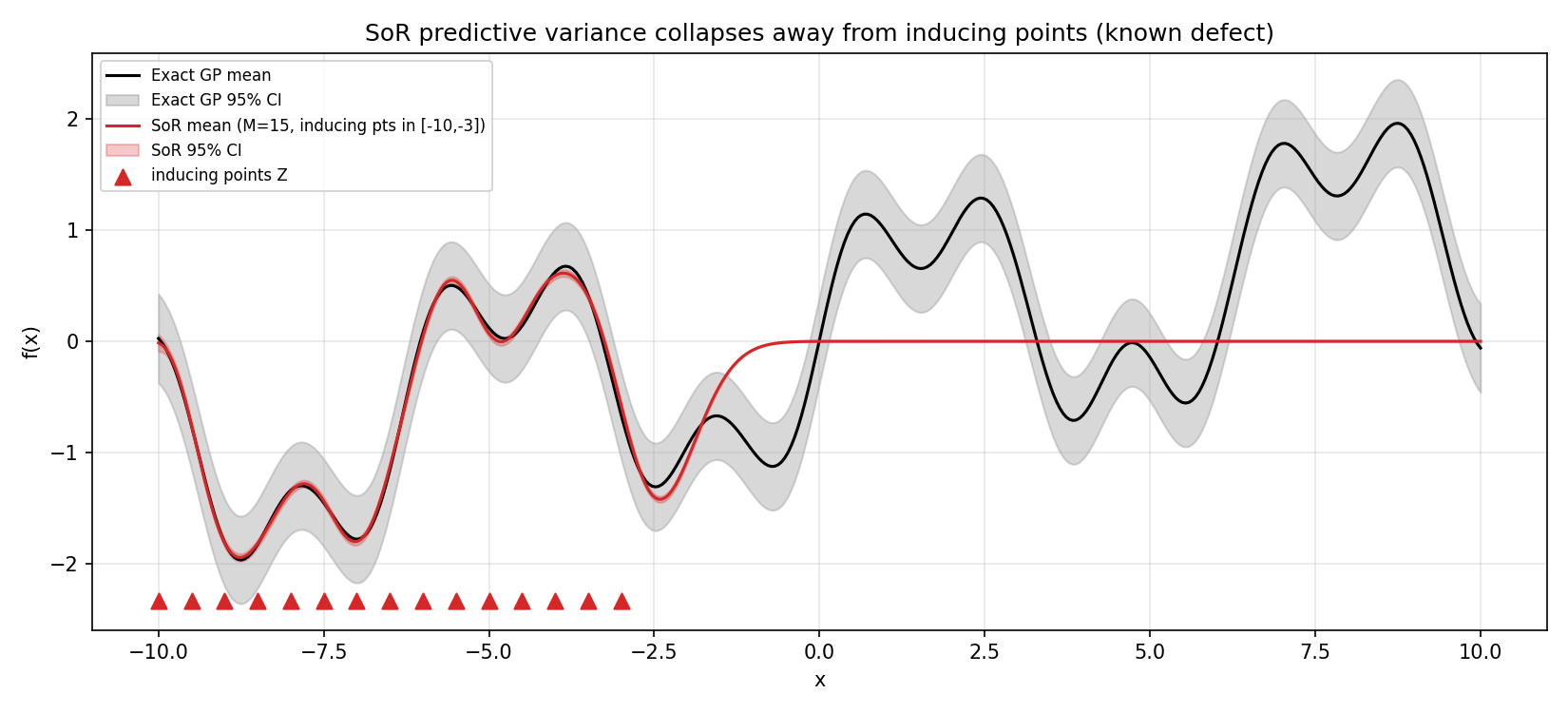
In the right half of the figure, SoR’s mean (red line) flattens to 0 and its confidence band (red shading) becomes essentially invisible, while the exact GP (black line, gray band) keeps tracking the true function’s variation. FITC (Snelson & Ghahramani, 2006) mitigates this defect with a diagonal correction; VFE (Titsias, 2009) goes further and optimizes the inducing-point locations themselves by maximizing a variational lower bound; SVGP (Hensman, Fusi & Lawrence, 2013) mini-batches VFE to scale past \(n \sim 10^6\) . These were mentioned by name only in the “Sparse GP Overview” section of https://yuhi-sa.github.io/en/posts/20260502_gaussian_process/1/ — understanding why SoR’s variance collapses, as we’ve now seen directly, makes it clear exactly what problem each of these later refinements is solving.
Summary: Practical Guidance
| Question | What the derivation and experiments show |
|---|---|
| Is the math correct? | SoR reduces exactly to the exact GP when \(m=n\) (differences of order \(10^{-9}\) ) |
| RMSE convergence | At \(n=5000\) , \(M=100\) (2% of training points) shrinks the gap to the exact GP to \(4\times10^{-7}\) |
| Speed | 337x faster at \(M=100\) , 2042x at \(M=10\) (with an accuracy trade-off) |
| Inducing-point placement | k-means ≈ uniform > random. Random has worse average accuracy and high seed-to-seed variance |
| Predictive variance | SoR’s variance collapses to 0 away from inducing points — a known defect. Use FITC or later if calibration matters |
| What’s next | FITC if you need calibrated variance, VFE if you want to optimize inducing points themselves, SVGP if \(n \gtrsim 10^5\) |
Our measurements confirm that SoR — the simplest inducing-point method to implement — can approximate the exact GP to high precision without ever forming an \(n \times n\) matrix. But its predictive variance has a real weakness, so if uncertainty estimates themselves feed into a decision (as in Bayesian optimization’s acquisition functions), it’s worth considering FITC or the VFE family instead.
Related Articles
- Gaussian Process Regression: Fundamentals and Python Implementation - The prerequisite for this article: the theory, derivation, and numerical stability of the exact GP.
- Gaussian Process Regression in Practice: Kernel Design and Applications - A practitioner’s overview of kernel design, hyperparameter optimization, and approximation methods including SoR. This article is a deep dive into the derivation and experiments behind the SoR snippet mentioned there.
- Bayesian Optimization: Fundamentals and Python Implementation - When a GP surrogate is evaluated hundreds to thousands of times, this article’s scalability discussion becomes directly relevant.
- SVM Kernel Design: Mercer’s Theorem, Gram Matrix Positive Semi-Definiteness, and Random Fourier Features - Random Fourier Features approximate the kernel matrix itself via an explicit low-rank feature map — a “relative” of inducing-point methods that attacks the same \(O(n^2)\) -\(O(n^3)\) wall from a different angle.
References
- Rasmussen, C. E., & Williams, C. K. I. (2006). Gaussian Processes for Machine Learning. MIT Press.
- Silverman, B. W. (1985). “Some Aspects of the Spline Smoothing Approach to Non-Parametric Regression Curve Fitting.” Journal of the Royal Statistical Society: Series B, 47(1), 1-21.
- Smola, A. J., & Bartlett, P. (2001). “Sparse Greedy Gaussian Process Regression.” NeurIPS 2000.
- Snelson, E., & Ghahramani, Z. (2006). “Sparse Gaussian Processes using Pseudo-inputs.” NeurIPS 2006. (FITC)
- Titsias, M. (2009). “Variational Learning of Inducing Variables in Sparse Gaussian Processes.” AISTATS 2009. (VFE)
- Hensman, J., Fusi, N., & Lawrence, N. D. (2013). “Gaussian Processes for Big Data.” UAI 2013. (SVGP)
- Quiñonero-Candela, J., & Rasmussen, C. E. (2005). “A Unifying View of Sparse Approximate Gaussian Process Regression.” Journal of Machine Learning Research, 6, 1939-1959.