Introduction
https://yuhi-sa.github.io/en/posts/20260223_bayesian_optimization/1/ covered how a Gaussian process surrogate combines with three acquisition functions – EI, UCB, and PI – to decide where to evaluate next. All three plug the GP’s predictive mean and variance into an explicit formula to pick the next point. This article covers a different approach: Thompson Sampling, which makes decisions by drawing a sample from a posterior distribution and acting on that sample directly. We start from the most fundamental setting where this idea applies – the multi-armed bandit problem. Thompson Sampling, proposed in 1933, is one of the oldest exploration strategies in the field, yet it remains a standard choice in modern recommendation systems, ad serving, and sequential A/B testing. In the second half, we implement it combined with a Gaussian process to show it also functions as an acquisition function for Bayesian optimization (GP-TS).
The Multi-Armed Bandit Problem
The multi-armed bandit (MAB) problem involves \(K\) “arms,” where pulling arm \(i\) yields a reward drawn from an unknown distribution – a sequential decision-making problem. This article uses the most basic variant, the Bernoulli bandit: pulling arm \(i\) returns a reward of 1 with probability \(p_i\) and 0 with probability \(1-p_i\) (with \(p_i\) unknown to the agent).
The goal over \(T\) steps is to maximize cumulative reward, which is equivalent to minimizing the cumulative regret:
\[ R(T) = \sum_{t=1}^{T} \left( p^* - p_{a_t} \right) \tag{1} \]where \(p^* = \max_i p_i\) is the success probability of the best arm and \(a_t\) is the arm chosen by the agent at time \(t\) . Equation (1) measures the gap between the reward that would have been earned by always pulling the best arm from the start and the reward actually obtained. A good algorithm keeps \(R(T)\) growing as slowly as possible – ideally \(O(\log T)\) .
The multi-armed bandit distills, in its simplest form, the central tension found throughout reinforcement learning and sequential experimental design: the trade-off between exploration (trying under-tested arms to gather information) and exploitation (repeatedly choosing the arm that currently looks best).
Three Strategies: Epsilon-Greedy, UCB1, and Thompson Sampling
Epsilon-Greedy
The simplest strategy: with probability \(1-\varepsilon\) , pick the arm with the highest empirical average so far (exploitation); with probability \(\varepsilon\) , pick a random arm (exploration).
\[ a_t = \begin{cases} \arg\max_i \hat{p}_i(t) & \text{with probability } 1-\varepsilon \\ \text{uniformly random arm} & \text{with probability } \varepsilon \end{cases} \tag{2} \]where \(\hat{p}_i(t)\) is the empirical success rate of arm \(i\) up to time \(t\) . Because \(\varepsilon\) is fixed, the algorithm keeps making “wasteful” random choices even after it has converged, so cumulative regret grows asymptotically as \(\Theta(T)\) (linear).
UCB1 (Upper Confidence Bound)
Based on the principle of “optimism in the face of uncertainty,” UCB1 scores each arm by its empirical mean plus a confidence-interval bonus:
\[ a_t = \arg\max_i \left( \hat{p}_i(t) + \sqrt{\frac{2\ln t}{n_i(t)}} \right) \tag{3} \]where \(n_i(t)\) is the number of times arm \(i\) has been pulled so far. Arms pulled fewer times get a larger bonus \(\sqrt{2\ln t / n_i(t)}\) , automatically driving exploration. UCB1 has a theoretical guarantee of \(O(\log T)\) cumulative regret (Auer, Cesa-Bianchi & Fischer, 2002).
Thompson Sampling
Thompson Sampling maintains a Bayesian posterior over each arm’s success probability \(p_i\) and draws one sample from each posterior, then pulls the arm whose sample is largest. Since the Beta distribution is the conjugate prior for Bernoulli rewards, the posterior for arm \(i\) updates in closed form:
\[ p_i \mid \mathcal{D} \sim \text{Beta}(\alpha_i, \beta_i), \qquad \alpha_i = 1 + s_i, \quad \beta_i = 1 + f_i \tag{4} \]where \(s_i, f_i\) are the number of successes and failures observed for arm \(i\) , and the prior is the uninformative \(\text{Beta}(1,1)\) (uniform) distribution. At each step:
\[ \theta_i \sim \text{Beta}(\alpha_i, \beta_i) \quad (i=1,\ldots,K), \qquad a_t = \arg\max_i \theta_i \tag{5} \]the arm with the largest sampled value is pulled, and \(\alpha_{a_t}\) or \(\beta_{a_t}\) in Eq. (4) is incremented depending on the outcome. This procedure has an elegant property: the spread of the posterior itself automatically regulates the amount of exploration. Arms with little data (wide, uncertain posteriors) produce more widely varying samples and get pulled more often; as data accumulates and a posterior concentrates around the true value, that arm naturally gets pulled less. The key contrast is that UCB1’s confidence bonus controls exploration through a fixed formula, whereas Thompson Sampling achieves the same effect through the stochastic mechanism of sampling from a Bayesian posterior.
Python Implementation
We implement all three methods from scratch in NumPy.
import numpy as np

def eps_greedy(rng, K, T, true_probs, eps=0.1):
    counts, sums = np.zeros(K), np.zeros(K)
    chosen = np.zeros(T, dtype=int)
    for t in range(T):
        if t < K:
            a = t  # pull each arm once before starting
        elif rng.random() < eps:
            a = rng.integers(K)
        else:
            a = np.argmax(sums / np.maximum(counts, 1))
        r = float(rng.random() < true_probs[a])
        counts[a] += 1
        sums[a] += r
        chosen[t] = a
    return chosen

def ucb1(rng, K, T, true_probs):
    counts, sums = np.zeros(K), np.zeros(K)
    chosen = np.zeros(T, dtype=int)
    for t in range(T):
        if t < K:
            a = t
        else:
            bonus = np.sqrt(2 * np.log(t + 1) / counts)
            a = np.argmax(sums / counts + bonus)
        r = float(rng.random() < true_probs[a])
        counts[a] += 1
        sums[a] += r
        chosen[t] = a
    return chosen

def thompson_sampling(rng, K, T, true_probs):
    alpha, beta = np.ones(K), np.ones(K)
    chosen = np.zeros(T, dtype=int)
    for t in range(T):
        theta = rng.beta(alpha, beta)   # Eq. (5): sample each arm's posterior
        a = np.argmax(theta)
        r = float(rng.random() < true_probs[a])
        if r > 0:
            alpha[a] += 1                # Eq. (4): update alpha on success
        else:
            beta[a] += 1                 # Eq. (4): update beta on failure
        chosen[t] = a
    return chosen
eps_greedy, ucb1, and thompson_sampling map directly to Eqs. (2), (3), and (4)-(5) respectively. Updates like counts[a] += 1 maintain each method’s running statistics online (empirical means, or the Beta distribution’s parameters).
Numerical Experiment: Comparing Cumulative Regret
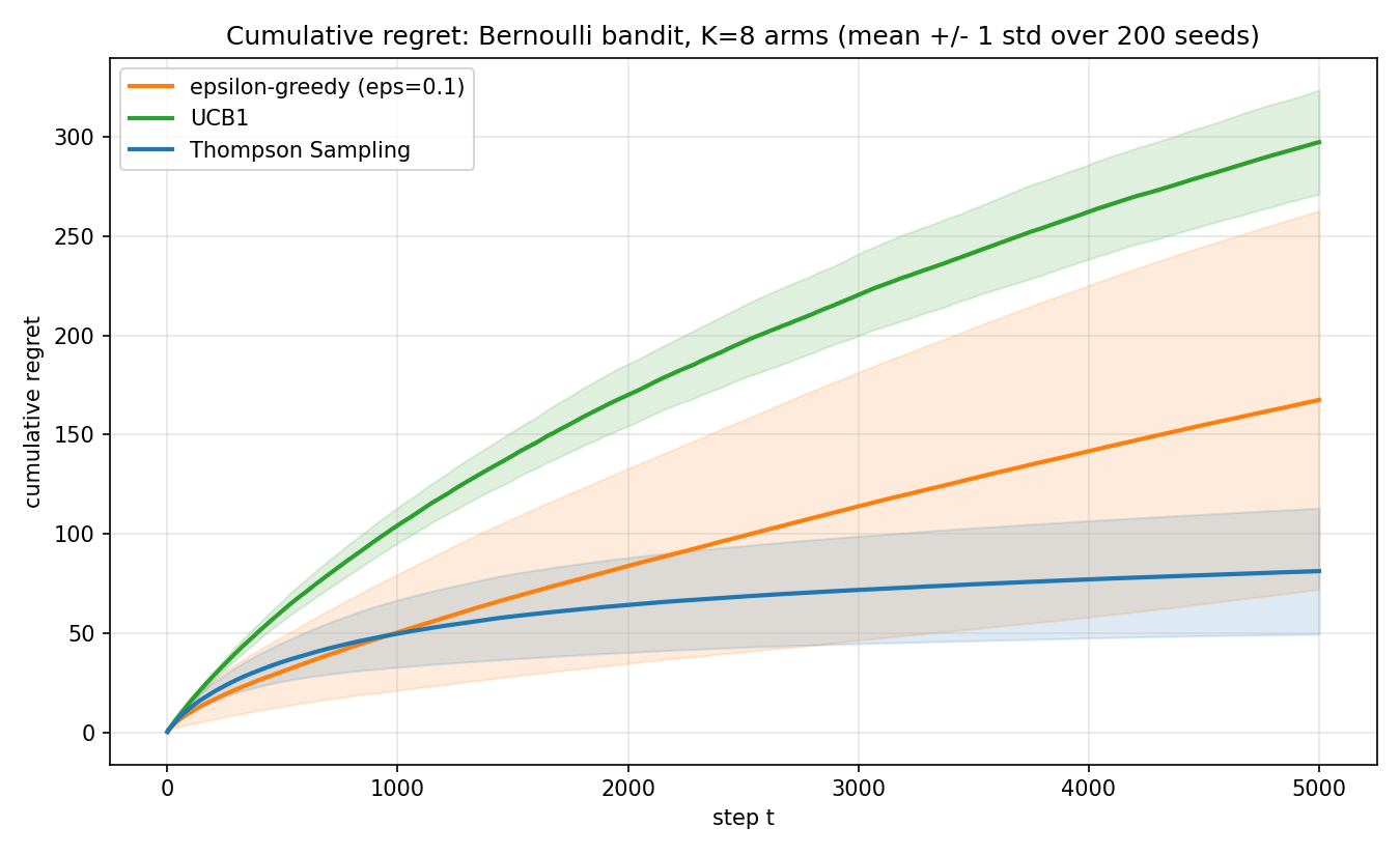
Using a Bernoulli bandit with \(K=8\)
arms and success probabilities \(p_i \in \{0.10, 0.20, 0.30, 0.35, 0.40, 0.45, 0.50, 0.55\}\)
(best arm \(p^*=0.55\)
), we compared cumulative regret (Eq. 1) over \(T=5000\)
steps, averaged across 200 seeds (seed=1000 through 1199).
K = 8
true_probs = np.array([0.10, 0.20, 0.30, 0.35, 0.40, 0.45, 0.50, 0.55])
T, N_SEEDS = 5000, 200
best_p = true_probs.max()

regret_curves = {name: np.zeros((N_SEEDS, T)) for name in
                  ["eps_greedy", "ucb1", "thompson"]}
for seed in range(N_SEEDS):
    for name, fn in [("eps_greedy", eps_greedy), ("ucb1", ucb1),
                      ("thompson", thompson_sampling)]:
        rng = np.random.default_rng(1000 + seed)
        chosen = fn(rng, K, T, true_probs)
        regret_curves[name][seed] = np.cumsum(best_p - true_probs[chosen])
Results
K=8 arms, true_probs=[0.1, 0.2, 0.3, 0.35, 0.4, 0.45, 0.5, 0.55], best_p=0.55
T=5000 steps, N_SEEDS=200

eps_greedy  : cumulative regret at T=5000: mean=167.53 std=95.31  %pulls on best arm=70.0%
ucb1        : cumulative regret at T=5000: mean=297.35 std=26.22  %pulls on best arm=51.7%
thompson    : cumulative regret at T=5000: mean=81.25 std=31.75  %pulls on best arm=84.2%
Thompson Sampling’s cumulative regret of 81.25 is about half that of epsilon-greedy (167.53), and roughly a quarter of UCB1’s (297.35). It also pulled the best arm most often (84.2%), ahead of epsilon-greedy (70.0%) and UCB1 (51.7%).
Looking at intermediate checkpoints shows how this gap opens up over time:
t=  100: eps_greedy=   10.14  ucb1=   15.56  thompson=   12.39
t=  500: eps_greedy=   30.68  ucb1=   61.23  thompson=   35.52
t= 1000: eps_greedy=   50.41  ucb1=  104.26  thompson=   49.75
t= 2000: eps_greedy=   83.82  ucb1=  169.98  thompson=   64.22
t= 5000: eps_greedy=  167.53  ucb1=  297.35  thompson=   81.25
At \(t=100\) , Thompson Sampling and epsilon-greedy are roughly tied, but Thompson Sampling pulls ahead around \(t=1000\) and the gap keeps widening. We can confirm this quantitatively by comparing each method’s “late-stage slope” (additional regret per step) between \(t\in[500,1000]\) and \(t\in[4000,5000]\) :
eps_greedy   slope[500:1000]=0.0395/step  slope[4000:5000]=0.0259/step
ucb1         slope[500:1000]=0.0860/step  slope[4000:5000]=0.0351/step
thompson     slope[500:1000]=0.0285/step  slope[4000:5000]=0.0041/step
Thompson Sampling’s slope shrinks roughly sevenfold, from 0.0285 to 0.0041, suggesting the regret growth is decelerating toward logarithmic behavior (consistent with the theoretical \(O(\log T)\) lower bound). Epsilon-greedy’s slope, by contrast, shrinks only about 1.5x (0.0395 to 0.0259) – the fixed exploration rate \(\varepsilon\) keeps forcing random exploration all the way through, so its slope never gets close to zero. This data alone cannot prove the tail is truly linear, but the contrast in how sharply the slope decays is unambiguous.
The fact that UCB1 underperforms epsilon-greedy in this experiment may look surprising at first, but the cause is that the gaps between arms’ success probabilities are small (at most 0.05). UCB1’s confidence bonus \(\sqrt{2\ln t/n_i(t)}\) is designed conservatively enough to hold for all arms under its theoretical guarantee, so under small gaps it keeps judging that it “isn’t confident enough yet” and re-pulls suboptimal arms; 5000 steps is not enough for it to fully converge here. With larger gaps (e.g., spacing \(p_i\) by 0.2), UCB1’s performance improves substantially.
Convergence of the Beta Posterior
We visualize the core mechanism behind Thompson Sampling: posterior updating. Fixing an arm with true success probability \(p=0.35\)
and pulling it repeatedly, we plot the Beta posterior \(\text{Beta}(1+s, 1+f)\)
at trial counts \(n \in \{0, 1, 5, 20, 100, 500\}\)
(seed=20260729).
from scipy.stats import beta as beta_dist

true_p = 0.35
rng = np.random.default_rng(20260729)
outcomes = (rng.random(500) < true_p).astype(int)
cum_successes = np.cumsum(outcomes)

for n in [0, 1, 5, 20, 100, 500]:
    s = cum_successes[n - 1] if n > 0 else 0
    f = n - s
    alpha, beta_param = 1 + s, 1 + f
    mean = alpha / (alpha + beta_param)
    print(f"n={n}: Beta({alpha},{beta_param})  mean={mean:.4f}")
n=   0  successes=   0  Beta(1,1)  mean=0.5000  std=0.2887
n=   1  successes=   1  Beta(2,1)  mean=0.6667  std=0.2357
n=   5  successes=   3  Beta(4,3)  mean=0.5714  std=0.1750
n=  20  successes=   7  Beta(8,14)  mean=0.3636  std=0.1003
n= 100  successes=  35  Beta(36,66)  mean=0.3529  std=0.0471
n= 500  successes= 188  Beta(189,313)  mean=0.3765  std=0.0216
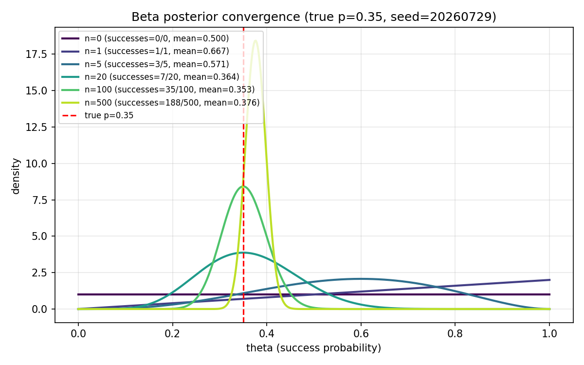
At \(n=0\) (uniform prior), the distribution is very spread out, with a standard deviation of 0.289. By \(n=20\) it has narrowed to 0.100, and by \(n=500\) to 0.022, with the posterior mean converging near the true value of 0.35 (at \(n=20\) the empirical rate happened to land exactly at 7/20=0.35, which is why the posterior mean 0.364 is already close to truth; note also that at \(n=1\) , an extreme single observation of 1/1=1.0 pulled the posterior mean to 0.667 – the \(\text{Beta}(1,1)\) prior tempers extreme values somewhat, but sizable swings remain unavoidable with very little data, a basic feature of Bayesian inference). This property – wide posteriors when data is scarce, natural convergence as data accumulates – is a direct visualization of how Thompson Sampling automatically balances exploration and exploitation.
Extension: Gaussian Process + Thompson Sampling (GP-TS)
The Bernoulli bandit above had a discrete, finite set of arms, but the Bayesian optimization covered in https://yuhi-sa.github.io/en/posts/20260223_bayesian_optimization/1/ operates over a continuous space \(\mathcal{X} \subseteq \mathbb{R}^d\) . Thompson Sampling’s idea extends naturally to this setting by replacing the discrete arms with a https://yuhi-sa.github.io/en/posts/20260502_gaussian_process/1/ as the surrogate model. This is GP-Thompson Sampling (GP-TS).
The GP-TS procedure is:
- Fit a Gaussian process to the observations so far \(\mathcal{D} = \{(\mathbf{x}_i, y_i)\}\)
- Sample one function from the GP posterior over a set of candidate points \(X_{\text{cand}}\) (this is a draw from a multivariate normal \(\mathcal{N}(\boldsymbol{\mu}, \boldsymbol{\Sigma})\) – the continuous-space analog of drawing one point from a Beta distribution in Eq. (5) for the bandit)
- Select the point that minimizes (or maximizes) the sampled function as the next evaluation point
Where EI, UCB, and PI substitute the predictive mean and variance into explicit formulas (Eqs. 7-10 in https://yuhi-sa.github.io/en/posts/20260223_bayesian_optimization/1/) to pick the next point, GP-TS is fundamentally different: it samples a realization from the posterior and optimizes that sample itself. Crucially, Eq. (6) requires not just the predictive variance at each point but the covariance between candidate points (the off-diagonal terms of the GP posterior). EI and the other acquisition functions only needed each point’s marginal variance, but GP-TS needs to sample “one internally consistent function across all candidate points,” which requires the full covariance matrix.
Python Implementation
class GaussianProcess:
    def __init__(self, length_scale=1.0, signal_var=1.0, noise_var=1e-6):
        self.l, self.sf2, self.sn2 = length_scale, signal_var, noise_var

    def kernel(self, X1, X2):
        dist_sq = (np.sum(X1**2, axis=1, keepdims=True)
                   - 2.0 * X1 @ X2.T + np.sum(X2**2, axis=1))
        return self.sf2 * np.exp(-0.5 * dist_sq / self.l**2)

    def fit(self, X, y):
        self.X_train, self.y_train = X.copy(), y.copy()
        K = self.kernel(X, X) + self.sn2 * np.eye(len(X))
        self.K_inv = np.linalg.inv(K)

    def predict_full_cov(self, X_new):
        """Predictive mean and *full* covariance matrix (needed for GP-TS's function sampling)"""
        k_star = self.kernel(self.X_train, X_new)
        mu = k_star.T @ self.K_inv @ self.y_train
        cov = self.kernel(X_new, X_new) - k_star.T @ self.K_inv @ k_star
        return mu, cov + 1e-8 * np.eye(len(X_new))  # jitter for numerical stability

def gp_thompson_step(gp, X_cand, rng):
    """Eq. (6): sample one function from the GP posterior and return its minimizer"""
    mu, cov = gp.predict_full_cov(X_cand)
    f_sample = rng.multivariate_normal(mu, cov)
    return X_cand[np.argmin(f_sample)]
The GaussianProcess class shares kernel and fit with the class in https://yuhi-sa.github.io/en/posts/20260223_bayesian_optimization/1/, but adds predict_full_cov (the entire covariance matrix) instead of predict (marginal variance only). gp_thompson_step implements Eq. (6), with rng.multivariate_normal corresponding to “drawing one function from the posterior.”
Numerical Experiment: Comparison with EI
Using the same test function as https://yuhi-sa.github.io/en/posts/20260223_bayesian_optimization/1/, \(f(x) = \sin(3x) + 0.1x^2 - 0.5\cos(7x)\)
, over \(x\in[-3,3]\)
, with 3 initial points plus 12 sequential evaluations (15 total), seed=42, we ran EI and GP-TS from identical initial points for comparison.
EI    : best_x=1.6894  best_f=-1.0210  regret=0.0172  n_evals=15
GP-TS : best_x=-0.7876  best_f=-0.9993  regret=0.0388  n_evals=15
The true global minimum is \(f(\mathbf{x}^*) = -1.038189\) (see https://yuhi-sa.github.io/en/posts/20260223_bayesian_optimization/1/), so in this single condition EI achieved a regret of 0.0172 versus GP-TS’s 0.0388 – EI found a solution closer to the true optimum.
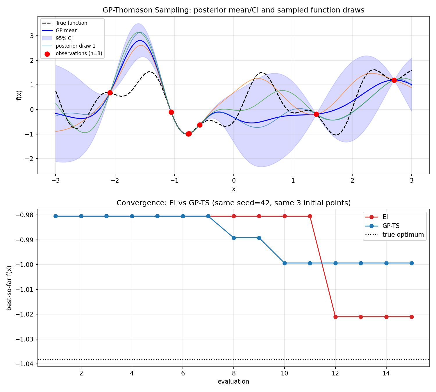
The top panel shows three functions sampled from the GP posterior built on 8 observations. Near the observed points (low uncertainty), all three samples converge close to the GP mean, while in sparsely observed regions (around \(x\in[-0.5, 1]\) ) the samples diverge widely. This “wide dispersion of sampled values in high-uncertainty regions” is exactly GP-TS’s exploration mechanism. The bottom panel shows how EI and GP-TS converge from the same initial points: in this particular run, GP-TS keeps improving at evaluations 8 and 10 and reaches \(f\approx-0.999\) faster than EI, but EI ultimately discovers a deeper minimum of \(-1.0210\) at evaluation 12.
Additional Multi-Seed Check
Drawing conclusions like “EI is better” from a single seed alone would be premature (as noted in the practical caveats of https://yuhi-sa.github.io/en/posts/20260223_bayesian_optimization/1/). We therefore reran the same setup (3 initial points, 12 sequential evaluations) over 30 seeds (seed=100 through 129) and examined the regret distribution.
n_seeds=30
EI    regret: mean=0.0146 median=0.0022 std=0.0174
GP-TS regret: mean=0.0640 median=0.0388 std=0.0918
GP-TS better in 26.7% of seeds
GP-TS beat EI (lower regret) in only 26.7% of the 30 seeds, and its average regret (0.0640) was about 4.4x larger than EI’s (0.0146). In this particular low-budget (15 evaluations), one-dimensional, weakly multimodal test-function setting, EI tends to find good solutions more robustly. This is likely because GP-TS, per Eq. (6), samples a single function and commits to its minimizer – an unlucky outlier draw sends it off in the wrong direction – whereas EI always picks the point of maximum expected improvement based on two deterministic statistics (mean and variance), which keeps variance lower when the evaluation budget is small. On the other hand, Thompson Sampling is known to perform competitively with (or better than) EI/UCB in settings with many sequential decisions, or where asynchronous/parallel evaluation is required (Chowdhury & Gopalan, 2017; Kandasamy et al., 2018), as we also saw for the bandit case above – so the “only 15 evaluations” setting used here is likely unfavorable to GP-TS specifically.
When to Use Thompson Sampling vs. UCB-Style Acquisition
Finally, we summarize how Thompson Sampling fits into practice based on what this article has shown.
| Epsilon-Greedy | UCB1 / UCB | Thompson Sampling | |
|---|---|---|---|
| Exploration mechanism | Fixed-rate random search | Fixed confidence-interval bonus | Sampling from the posterior |
| Implementation effort | Simplest | Simple (closed-form) | Moderate (posterior bookkeeping) |
| Theoretical regret | \(\Theta(T)\) (linear) | \(O(\log T)\) | \(O(\log T)\) (Bernoulli case) |
| Parallel/batch queries | Easy | Requires extra care | Extends naturally (multiple draws) |
| Continuous extension | Easy but inefficient | Guarantees become complex | Extends naturally as GP-TS (this article) |
Thompson Sampling’s practical strength is that it extends naturally to batch settings where multiple candidates must be evaluated in parallel. UCB-style methods pick one point deterministically, so ensuring diversity across a batch requires extra machinery; Thompson Sampling naturally produces a diverse set of candidates simply by drawing multiple independent samples from the posterior (each with a different random seed). This is why it is widely adopted in production online-learning systems that handle large volumes of parallel requests, such as ad serving and recommendation systems (Chapelle & Li, 2011; Russo et al., 2018).
Summary
- We implemented three multi-armed bandit strategies (epsilon-greedy, UCB1, Thompson Sampling) from scratch in NumPy and compared cumulative regret on a Bernoulli bandit with \(K=8\) arms over \(T=5000\) steps, averaged across 200 seeds. Thompson Sampling achieved the lowest cumulative regret (81.25), about half of epsilon-greedy (167.53) and roughly a quarter of UCB1 (297.35).
- The core of Thompson Sampling is maintaining a Beta posterior \(\text{Beta}(1+s,1+f)\) over each arm’s success probability and picking the arm with the largest sample. We confirmed empirically that as trials grew from 0 to 500, the posterior’s standard deviation monotonically shrank from 0.289 to 0.022.
- GP-Thompson Sampling extends this idea to continuous-space optimization using a Gaussian process. In a single-condition test with a 30-seed follow-up check on a Bayesian optimization test function, EI achieved a lower average regret than GP-TS in this low-evaluation-budget (15 evaluations) setting (0.0146 vs. 0.0640) and proved more robust. This result is specific to the low-budget, low-dimensional condition tested; Thompson Sampling is known to become competitive or superior in settings involving many sequential decisions.
Related Articles
- Bayesian Optimization: Fundamentals and Python Implementation - GP-TS in this article stands as a fourth acquisition function alongside EI, UCB, and PI covered there.
- Gaussian Process Regression: Theory and Python Implementation - The theoretical foundation of the Gaussian process surrogate used by GP-TS.
- Gaussian Process Regression in Practice: Kernel Design and Applications - Production-grade GP implementation details, including numerically stable Cholesky-based prediction.
- Hamiltonian Monte Carlo (HMC) in Python - Extends the idea of sampling from a posterior to make it efficient in higher-dimensional, highly correlated distributions.
- Monte Carlo Optimization Methods Comparison (CEM/SA/GA/MPPI/PSO) - Hub article comparing sampling-based optimizers side by side.
References
- Thompson, W. R. (1933). On the likelihood that one unknown probability exceeds another in view of the evidence of two samples. Biometrika, 25(3/4), 285-294.
- Auer, P., Cesa-Bianchi, N., & Fischer, P. (2002). Finite-time analysis of the multiarmed bandit problem. Machine Learning, 47(2-3), 235-256.
- Chapelle, O., & Li, L. (2011). An empirical evaluation of Thompson sampling. NeurIPS 2011.
- Russo, D. J., Van Roy, B., Kazerouni, A., Osband, I., & Wen, Z. (2018). A tutorial on Thompson sampling. Foundations and Trends in Machine Learning, 11(1), 1-96.
- Chowdhury, S. R., & Gopalan, A. (2017). On kernelized multi-armed bandits. ICML 2017.
- Kandasamy, K., Krishnamurthy, A., Schneider, J., & Póczos, B. (2018). Parallelised Bayesian optimisation via Thompson sampling. AISTATS 2018.