Introduction
In Bayesian Optimization Basics we covered the framework of maximizing acquisition functions (EI, UCB, PI) over a Gaussian-process surrogate. Yet the default sampler of Optuna , the most widely used hyperparameter tuning library in practice, is not a GP but TPE (Tree-structured Parzen Estimator).
Because optuna.create_study() just works, few people ever look inside TPE — which is a pity, since its idea is a neat inversion of GP-based Bayesian optimization. In this article we:
- Derive TPE’s core criterion — maximizing the density ratio \(l(x)/g(x)\) — from the EI formula
- Build a ~40-line from-scratch TPE with
scipy.stats.gaussian_kdeand visualize its internal state - Benchmark random search, TPE, multivariate TPE, and GP-EI on the Branin function over 30 seeds
- Measure the real-world payoff of tuning HistGradientBoosting on breast_cancer
All numbers below are measured, including the honest negative result that our naive TPE loses to random search in 1D.
How TPE Works: Flipping the Acquisition Function with Bayes’ Rule
A different viewpoint from GP-based Bayesian optimization
GP-based Bayesian optimization models \(p(y \mid x)\) : given an input, predict the distribution of the objective. TPE models the reverse. It splits the observation history by objective value and estimates
\[ p(x \mid y) = \begin{cases} l(x) & (y < y^{*}) \\ g(x) & (y \geq y^{*}) \end{cases} \tag{1} \]i.e., the distribution of inputs that produced good values \(l(x)\) and the distribution of inputs that produced bad values \(g(x)\) . The threshold \(y^{*}\) is the lower \(\gamma\) -quantile of observed values (for minimization; Optuna’s default \(\gamma\) varies with the number of trials, roughly the top 10–25%).
Maximizing EI is equivalent to maximizing the density ratio
The beauty of this formulation is that Expected Improvement turns into a density ratio via Bayes’ rule. Starting from the definition
\[ \mathrm{EI}_{y^{*}}(x) = \int_{-\infty}^{y^{*}} (y^{*} - y)\, p(y \mid x)\, dy \tag{2} \]substituting \(p(y \mid x) = p(x \mid y)\,p(y)/p(x)\) with \(p(x) = \gamma\, l(x) + (1 - \gamma)\, g(x)\) yields (see Bergstra et al., 2011 for the full derivation)
\[ \mathrm{EI}_{y^{*}}(x) \propto \left( \gamma + \frac{g(x)}{l(x)} (1 - \gamma) \right)^{-1} \tag{3} \]Since \((3)\) is monotonically decreasing in \(g(x)/l(x)\) , the point that maximizes EI is exactly the point that maximizes \(l(x)/g(x)\) . One TPE iteration is therefore just:
- Split observations into the top \(\gamma\) (good) and the rest (bad)
- Estimate \(l(x)\) and \(g(x)\) with Parzen windows (kernel density estimation)
- Sample candidates from \(l(x)\) and evaluate the one with the largest \(l(x)/g(x)\)
No \(O(n^3)\)
matrix algebra anywhere. The “tree-structured” part of the name refers to conditional (tree-shaped) search spaces — e.g., a suggest_int whose value decides which further suggest_float calls exist — which TPE handles naturally by keeping independent one-dimensional densities per node. Categorical parameters work too: density estimation degenerates to category frequencies.
A From-scratch Implementation in ~40 Lines
We implement the three steps with scipy.stats.gaussian_kde on the multimodal 1-D function
whose global minimum, from a 20,001-point grid, is \(f(1.483) = -0.904\) (with a local minimum trap near \(x \approx -0.5\) ).
import numpy as np
from scipy.stats import gaussian_kde


def f(x):
    return np.sin(3 * x) + 0.5 * x**2 - 0.7 * x


XLO, XHI = -2.0, 3.0


def tpe_minimize(n_trials=30, n_init=8, gamma=0.25, n_cand=24, seed=0):
    rng = np.random.default_rng(seed)
    xs, ys = [], []
    for i in range(n_trials):
        if i < n_init:  # random initialization
            x = rng.uniform(XLO, XHI)
        else:
            order = np.argsort(ys)
            n_good = max(2, int(np.ceil(gamma * len(ys))))
            good = np.array(xs)[order[:n_good]]   # good observations (top γ)
            bad = np.array(xs)[order[n_good:]]    # bad observations (rest)
            l = gaussian_kde(good, bw_method=0.35)
            g = gaussian_kde(bad, bw_method=0.35)
            cand = l.resample(n_cand, seed=rng.integers(1 << 31)).ravel()
            cand = np.clip(cand, XLO, XHI)
            x = cand[np.argmax(l(cand) / np.maximum(g(cand), 1e-12))]
        xs.append(float(x))
        ys.append(float(f(x)))
    return np.array(xs), np.array(ys)
The figure below visualizes the internal state after 20 trials of one seed.
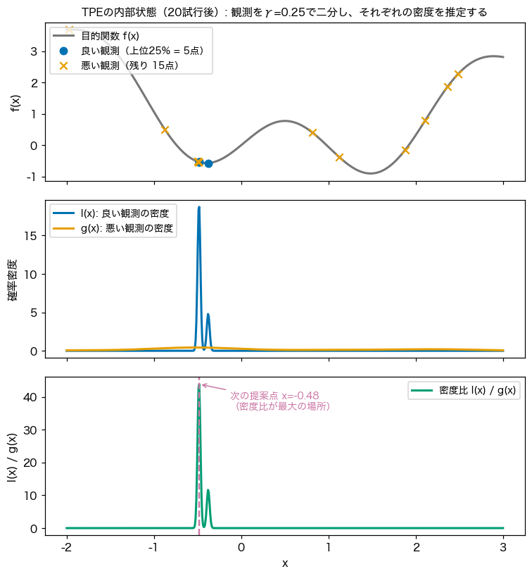
You can see TPE’s behavior directly — “sample where good observations concentrate, avoid where bad ones do” — and also that this run is stuck at the local minimum \(x \approx -0.5\) . Once good observations cluster around a local optimum, \(l(x)\) peaks there and so do the proposals: the classic weakness of naive TPE.
The honest result: these 40 lines lose to random search
Over 50 seeds × 30 trials, the gap between the best value found and the global minimum:
| Method | Mean gap (50 seeds) | Std |
|---|---|---|
| From-scratch TPE | 0.206 | 0.212 |
| Random search | 0.046 | 0.073 |
Random search wins decisively. In a 1-D interval of width 5, thirty uniform samples almost surely land near the global optimum, while the naive TPE’s average is dragged down by seeds that lock onto the local minimum. Sampling candidates only from \(l(x)\) provides no exploration mechanism at all.
Optuna’s TPESampler layers several fixes on top of the skeleton:
- Prior mixing: blend a prior component covering the whole search space into \(l(x)\) and \(g(x)\) so no region has zero density (already present in Bergstra’s original paper)
- Bandwidth rules adapted to sample count and range
n_startup_trials(default 10): let early trials be purely random- Multivariate TPE: replace independent per-parameter KDEs with a multivariate KDE that captures correlations (benchmarked below)
The main lesson of writing TPE yourself: the skeleton fits in 40 lines, but the practical performance lives in the engineering around it.
Branin Benchmark: TPE vs GP-EI vs Random
The picture changes with dimensionality. On the standard Branin benchmark (2-D, global minimum \(0.397887\) ) we compare mean convergence over 60 trials × 30 seeds, using Optuna 4.9.0.
import optuna

optuna.logging.set_verbosity(optuna.logging.WARNING)


def branin(x1, x2):
    a, b, c = 1.0, 5.1 / (4 * np.pi**2), 5 / np.pi
    r, s, t = 6.0, 10.0, 1 / (8 * np.pi)
    return a * (x2 - b * x1**2 + c * x1 - r) ** 2 + s * (1 - t) * np.cos(x1) + s


def objective(trial):
    x1 = trial.suggest_float("x1", -5, 10)
    x2 = trial.suggest_float("x2", 0, 15)
    return branin(x1, x2)


samplers = {
    "random": lambda s: optuna.samplers.RandomSampler(seed=s),
    "tpe": lambda s: optuna.samplers.TPESampler(seed=s),
    "tpe_mv": lambda s: optuna.samplers.TPESampler(seed=s, multivariate=True),
}
study = optuna.create_study(sampler=samplers["tpe"](0))
study.optimize(objective, n_trials=60)
The GP-EI baseline is our own sklearn GaussianProcessRegressor (Matérn 5/2) + EI maximization, in the same style as the Bayesian optimization article.
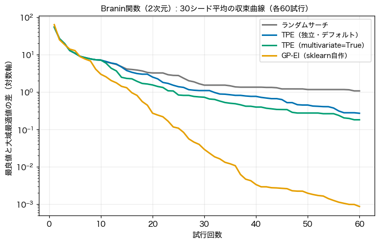
| Method | Gap after 20 trials | Gap after 60 trials (± std) |
|---|---|---|
| Random search | 3.20 | 1.061 ± 0.987 |
| TPE (default, independent) | 2.49 | 0.268 ± 0.304 |
| TPE (multivariate=True) | 1.53 | 0.180 ± 0.143 |
| GP-EI (from scratch) | 0.27 | 0.0009 ± 0.0010 |
Three observations:
- TPE clearly beats random search (roughly 4–6× smaller gap) — the advantage that was absent in 1D appears in 2D.
multivariate=Trueis a free win. On functions with correlated inputs like Branin it converges consistently faster than independent TPE with less than half the variance. It is still off by default in Optuna, so it is worth enabling for mostly-continuous spaces.- GP-EI dominates on low-dimensional, continuous, smooth problems — two orders of magnitude better than TPE after 60 trials.
Optuna still defaults to TPE because real tuning problems are rarely “low-dimensional, continuous, smooth”. Tree-shaped spaces with categorical choices (optimizer type) and conditional parameters (per-layer widths that exist only for the chosen depth) do not fit a GP naturally, but TPE handles them out of the box. And where a GP refits with \(O(n^3)\) cost every trial, TPE only evaluates KDEs, staying cheap as trials accumulate.
Real-data Payoff: breast_cancer × HistGradientBoosting
Finally, how much does tuning actually buy? We tune four parameters of HistGradientBoostingClassifier on breast_cancer (569 samples), maximizing 5-fold CV ROC-AUC, with 40 trials × 5 seeds.
from sklearn.datasets import load_breast_cancer
from sklearn.ensemble import HistGradientBoostingClassifier
from sklearn.model_selection import cross_val_score

X, y = load_breast_cancer(return_X_y=True)


def objective(trial):
    model = HistGradientBoostingClassifier(
        learning_rate=trial.suggest_float("learning_rate", 0.01, 0.5, log=True),
        max_iter=trial.suggest_int("max_iter", 50, 300),
        max_leaf_nodes=trial.suggest_int("max_leaf_nodes", 7, 63),
        l2_regularization=trial.suggest_float("l2_regularization", 1e-6, 1.0, log=True),
        random_state=0,
    )
    return cross_val_score(model, X, y, cv=5, scoring="roc_auc").mean()


study = optuna.create_study(direction="maximize", sampler=optuna.samplers.TPESampler(seed=0))
study.optimize(objective, n_trials=40)
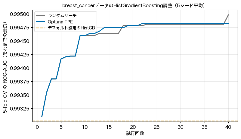
| Setting | 5-fold CV ROC-AUC |
|---|---|
| Default HistGB | 0.99302 |
| Random search (40 trials) | 0.99498 ± 0.00041 |
| Optuna TPE (40 trials) | 0.99482 ± 0.00026 |
Honestly reported: the difference between TPE and random search is within noise here (random’s mean is even marginally higher). The reason is clear — the defaults are already strong and a wide region of the parameter space performs equally well, so either method hits the ceiling (+0.002) within about 10 trials.
This does not mean tuning is pointless. It means sampler differences show up when the search space is large, evaluations are expensive enough that you must budget trials, or parameters interact strongly — exactly what the Branin experiment demonstrated. Conversely, treat with suspicion any benchmark that shows dramatic TPE-vs-random gains on an easy problem like this one.
Summary
| Item | Takeaway |
|---|---|
| Core of TPE | Split observations at the top \(\gamma\) ; pick the next point by maximizing \(l(x)/g(x)\) , which is equivalent to maximizing EI |
| Difference from GP | Models \(p(x \mid y)\) instead of \(p(y \mid x)\) ; no \(O(n^3)\) ; categorical and conditional spaces come for free |
| The 40-line version | Loses to random search in 1D (gap 0.206 vs 0.046, 50 seeds); practical performance lives in prior mixing and other fixes |
| Branin (2-D) | Gap: random 1.06 > TPE 0.27 > TPE-mv 0.18 ≫ GP-EI 0.0009; GP wins big on low-dim continuous problems |
| multivariate=True | Consistent improvement with correlated inputs (half the variance); worth enabling for continuous spaces |
| Real-data reality | With strong defaults on an easy dataset, 40-trial TPE ≈ random (+0.002 AUC either way) |
Related Articles
- Bayesian Optimization Basics and Python Implementation - The starting point of this article: GP surrogates and the EI/UCB/PI framework, including the EI definition in Eq. \((2)\) .
- Thompson Sampling: Theory and Python Implementation - The “fourth acquisition function” that picks points by sampling from the posterior — like TPE, a distribution-based selection rule.
- Gaussian Process Regression: Theory and Python Implementation - The surrogate model behind the GP-EI baseline used in this article.
- Sparse Gaussian Process Regression (Inducing Points) - Another answer to the GP’s \(O(n^3)\) problem: TPE sidesteps it by changing the model, sparse GPs by approximating it.
- Ensemble Learning (Random Forest / Gradient Boosting)
- Theory of the GBDT models tuned in the real-data experiment, including what
learning_rateandmax_leaf_nodesdo.
References
- Bergstra, J., Bardenet, R., Bengio, Y., & Kégl, B. (2011). “Algorithms for Hyper-Parameter Optimization”. Advances in Neural Information Processing Systems 24 (NIPS 2011).
- Akiba, T., Sano, S., Yanase, T., Ohta, T., & Koyama, M. (2019). “Optuna: A Next-generation Hyperparameter Optimization Framework”. Proceedings of the 25th ACM SIGKDD.
- Watanabe, S. (2023). “Tree-Structured Parzen Estimator: Understanding Its Algorithm Components and Their Roles for Better Empirical Performance”. arXiv:2304.11127
- Optuna documentation — TPESampler