A signal with amplitude 2, but an FFT peak below 2
Applying a Hann window can make an FFT peak look half as large. Increasing the FFT length can make it smaller again if the denominator is wrong. Before interpreting those changes as a fault in the measured signal, check normalization, one-sided scaling, and window gain.
This tutorial focuses on reading the peak amplitude of an isolated sinusoid in the input’s physical units. A voltage input gives an amplitude axis in volts. See the FFT introduction for transform algorithms, and window selection and PSD estimation for broader window comparisons.
Fix the amplitude convention first. In \(x[n]=A\cos(2\pi f_0 n/f_s+\phi)\) , \(A\) is peak amplitude. For an ordinary sinusoid well below Nyquist, RMS amplitude is \(A/\sqrt{2}\) and peak-to-peak amplitude is \(2A\) . The function below returns neither RMS amplitude nor power spectral density.
What needs to be corrected?
Let \(N\)
be the observed sample count, \(M\geq N\)
the FFT length after padding, and \(w[n]\)
the window. NumPy’s norm="backward" leaves the forward transform unscaled, so it computes
With a rectangular window, a sinusoid at an ordinary positive-frequency bin \(k_0f_s/N\) contributes \(NA/2\) to that bin. The other half belongs to its negative-frequency conjugate. A one-sided spectrum combines those contributions and reads \(2|X[k_0]|/N\) .
A window attenuates a bin-centered component according to its mean value. This mean is the coherent gain:
\[ G_c=\frac{1}{N}\sum_{n=0}^{N-1}w[n],\qquad \widehat A[k]=\frac{2|X_w[k]|}{NG_c}=\frac{2|X_w[k]|}{\sum_n w[n]}. \]This correction assumes an isolated, bin-centered sinusoid. It is not universally exact when the positive and negative window lobes overlap near DC or Nyquist, or when another nearby signal contributes to the same peak.
Do not hard-code a factor of two for every Hann window
scipy.signal.windows.hann(N, sym=False) produces a periodic window for spectral analysis. For \(N>1\)
, its sum is \(N/2\)
. The default sym=True produces a symmetric window for filter design, whose sum differs at the same length.
Compute the sum of the window you actually used, rather than inferring it from a window name. The SciPy Hann documentation explains the two conventions and their intended uses.
DC, Nyquist, and odd FFT lengths
rfft returns only the nonnegative-frequency part of a real-input transform. DC has no separate negative-frequency partner, so it must not be doubled.
| Bin | One-sided multiplier | Reason |
|---|---|---|
| DC (\(k=0\) ) | 1 | A single component |
| Ordinary positive frequency | 2 | Combines a negative-frequency conjugate |
| Final bin when \(M\) is even | 1 | The Nyquist component at \(f_s/2\) |
| Final bin when \(M\) is odd | 2 | An ordinary positive frequency below \(f_s/2\) |
Use FFT length \(M\)
, rather than original record length \(N\)
, for this decision. Padding an odd record to an even length creates an output with a Nyquist bin. The
NumPy rfft documentation
specifies the even/odd distinction.
The Nyquist test below uses \(A(-1)^n\) . At exactly \(f_s/2\) , samples depend on phase: a sine with phase zero produces only zeros. Those samples cannot identify the amplitude of an arbitrary-phase continuous sinusoid.
A reusable amplitude-spectrum function
The examples require Python, NumPy, SciPy, and Matplotlib. Paste both code blocks into the same file, in order, to run the assertions and save the figure.
import numpy as np
import matplotlib.pyplot as plt
from scipy.signal.windows import hann


def amplitude_spectrum(x, fs, window=None, nfft=None):
    x = np.asarray(x)
    if x.ndim != 1 or x.size < 2 or np.iscomplexobj(x):
        raise ValueError("x must be a real one-dimensional record")
    x = x.astype(float)
    n = len(x)
    if not np.isfinite(fs) or fs <= 0 or not np.all(np.isfinite(x)):
        raise ValueError("finite samples and positive fs are required")
    m = n if nfft is None else int(nfft)
    if m < n or (nfft is not None and m != nfft):
        raise ValueError("nfft must be an integer >= len(x)")
    w = np.ones(n) if window is None else np.asarray(window, dtype=float)
    if w.shape != x.shape or not np.all(np.isfinite(w)) or w.sum() <= 0:
        raise ValueError("window must match x and have a positive sum")
    z = np.fft.rfft(x * w, n=m, norm="backward")
    a = np.abs(z) / w.sum()
    if m % 2 == 0:
        a[1:-1] *= 2
    else:
        a[1:] *= 2
    f = np.fft.rfftfreq(m, d=1 / fs)
    return f, a


fs, amplitude = 1024.0, 2.0
for n in (1024, 1023):
    k = 37
    t = np.arange(n) / fs
    x = amplitude * np.cos(2 * np.pi * (k * fs / n) * t + 0.3)
    for w in (np.ones(n), hann(n, sym=False)):
        for m in (n, 4 * n):
            f, a = amplitude_spectrum(x, fs, w, m)
            np.testing.assert_allclose(a[k * (m // n)], amplitude, atol=1e-10)
    # DC is not doubled, for either record length.
    _, dc = amplitude_spectrum(np.full(n, 1.25), fs)
    np.testing.assert_allclose(dc[0], 1.25, atol=1e-12)
    print(f"N={n}: rectangular/Hann and padded amplitude checks passed")

# An even FFT has a Nyquist bin; an odd FFT has an ordinary final bin.
n = 1024
_, a = amplitude_spectrum(0.7 * (-1.0) ** np.arange(n), fs)
np.testing.assert_allclose(a[-1], 0.7, atol=1e-12)
n = 1023
k = n // 2
_, a = amplitude_spectrum(0.7 * np.cos(2 * np.pi * k * np.arange(n) / n), fs)
np.testing.assert_allclose(a[-1], 0.7, atol=1e-10)
The assertions combine rectangular and periodic Hann windows, even and odd records, and fourfold zero padding. The chosen bin-centered sinusoid still has a peak amplitude of 2. The final tests verify that an even FFT’s Nyquist bin is not doubled, while an odd FFT’s final bin is doubled.
The function does not remove DC automatically. If mean removal is appropriate, pass x - x.mean() before windowing, and distinguish this operation from measuring the DC value. Removing the mean can itself affect low-frequency estimates, so it should not be mandatory preprocessing for every signal.
Zero padding and off-bin peaks
A one-second record with \(N=256\) and \(f_s=256\) Hz has native FFT points spaced 1 Hz apart. A sinusoid at 10.5 Hz lies between the 10 Hz and 11 Hz bins. Neither bin samples the peak center.
Coherent gain correction does not remove this scalloping loss. Increasing the FFT length to 2048 gives a display grid spaced 0.125 Hz apart, which includes 10.5 Hz in this particular example.
# Off-bin sinusoid: compare native and padded frequency grids.
n, fs, f0, amplitude = 256, 256.0, 10.5, 2.0
t = np.arange(n) / fs
x = amplitude * np.cos(2 * np.pi * f0 * t + 0.3)
w = hann(n, sym=False)
fig, ax = plt.subplots(figsize=(8, 4.5))
for m, label, marker in ((n, "256-point FFT", "o"), (8 * n, "2048-point FFT", None)):
    f, a = amplitude_spectrum(x, fs, w, m)
    ax.plot(f, a, marker=marker, label=label)
    band = (f > 5) & (f < 16)
    idx = np.flatnonzero(band)[np.argmax(a[band])]
    print(f"M={m}: peak={a[idx]:.6f} at {f[idx]:.3f} Hz")
ax.axhline(amplitude, color="black", linestyle="--", label="True peak amplitude = 2")
ax.set(xlim=(6, 15), ylim=(0, 2.2), xlabel="Frequency [Hz]", ylabel="Peak amplitude",
       title="Same 1-second record, different FFT grids (periodic Hann)")
ax.grid(alpha=0.3)
ax.legend()
fig.tight_layout()
fig.savefig("amplitude_padding.png", dpi=170)
plt.close(fig)
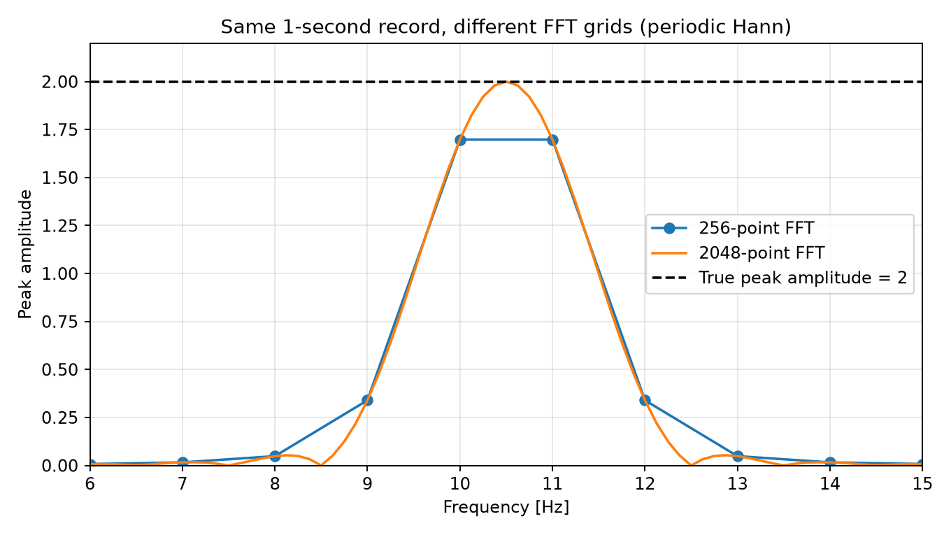
The maximum is approximately 1.698 before padding and 2.000 afterward. No additional observations were collected: the same windowed signal’s spectrum was evaluated at more frequency points. An arbitrary sinusoid’s frequency will not necessarily match a padded bin center.
Dividing by m, or by the padded length multiplied by the original window’s mean, would underestimate amplitude by a factor of eight here. The denominator remains the sum of the window applied to the original 256 samples.
Grid spacing is different from resolving two signals
- FFT frequency-point spacing is \(f_s/M\) .
- Observation duration is \(T=N/f_s\) and does not change with padding.
- Separating nearby frequencies depends on observation duration, window lobe width, signal strengths, noise, and other conditions.
Zero padding helps read a peak, but it does not guarantee that two nearby sinusoids become separable. If separation is the goal, consider collecting a longer record first. A sinusoid centered on an original FFT bin and a densely sampled padded frequency grid are different conditions.
When a peak is not an amplitude measurement
| Situation or goal | Appropriate response |
|---|---|
| Isolated bin-centered sinusoid | Correct by the window sum and respect one-sided exceptions |
| Isolated off-bin sinusoid | Consider padding, peak interpolation, or frequency estimation followed by sinusoidal fitting |
| Multiple nearby sinusoids | Do not treat one bin’s maximum as each signal’s amplitude; examine observation duration and separation |
| Broadband noise | Consider PSD and integration over a frequency band |
| Time-varying signal | Consider segment analysis rather than interpreting a whole-record FFT peak as a constant amplitude |
PSD uses a different normalization involving the sum of squared window values. Do not reuse the amplitude denominator for PSD. Changing the FFT to norm="forward" or "ortho" also changes transform scaling, so the denominator in this implementation would need adjustment.
Frequently asked questions
What should I divide FFT magnitudes by?
With NumPy’s default normalization and a real input, divide the windowed FFT magnitude by the sum of the original window. Double the one-sided values except DC and the Nyquist bin of an even-length FFT. This corrects an isolated bin-centered sinusoid; it does not guarantee an accurate amplitude for every peak.
Does zero padding change the amplitude normalization denominator?
No. Use the sum of the window applied to the observed samples. Dividing by the longer padded FFT length underestimates the amplitude.
Why is my Hann-windowed amplitude still too small after correction?
A frequency between FFT bins can suffer scalloping loss because the frequency grid misses the peak center. Coherent gain correction alone cannot remove this loss or interference from nearby signals.
Related articles
FFT theory and Python implementation : Transform definitions and basic analysis
Window selection and Welch PSD estimation : Measuring noise and power
DTFT, DFT, and FFT compared : Continuous frequency functions and sampled frequency points
Choosing Welch parameters : Segment length, overlap, and PSD units
References
- NumPy: numpy.fft.rfft : Padding, normalization, and even/odd output conventions
- NumPy: Discrete Fourier Transform : FFT APIs
- SciPy: scipy.signal.windows.hann : Periodic and symmetric windows