welch(x, fs=fs) estimates a PSD with very little code. It does not answer whether 256-sample segments are long enough, whether nfft=8192 can separate nearby tones, or how to convert a PSD peak into power.
This tutorial builds on window functions and PSD estimation and focuses on parameter decisions and numerical checks. Rather than comparing window families again, we will connect measurement requirements to the settings and test their consequences.
Start with segment duration, not FFT length
Let the full record contain \(N\) samples, the sample rate be \(f_s\) , the segment length be \(L\) , and overlap be \(O\) .
\[ T_{\mathrm{seg}} = \frac{L}{f_s}, \qquad H=L-O, \qquad K=1+\left\lfloor\frac{N-L}{H}\right\rfloor \]\(H\) is the hop between segment starts. \(K\) counts complete segments when an incomplete tail is discarded. These expressions assume \(N\ge L\) and \(0\le O<L\) .
| Parameter | Main effect | Consequence of increasing it |
|---|---|---|
nperseg=L | Segment duration and window frequency width | Better separation of nearby peaks, but fewer averages for a fixed record |
noverlap=O | Hop between segment starts | More segments and computation; correlated estimates require care |
nfft=M | Output frequency grid | Spacing becomes \(f_s/M\) ; observation duration stays unchanged |
For \(f_s=1024\) Hz, \(N=32768\) , and 50% overlap:
nperseg | nfft | Segment duration | Frequency spacing | Segments |
|---|---|---|---|---|
| 512 | 512 | 0.5 s | 2 Hz | 127 |
| 512 | 8192 | 0.5 s | 0.125 Hz | 127 |
| 4096 | 8192 | 4 s | 0.125 Hz | 15 |
The last two settings have identical frequency grids but different resolving power.
nperseg: work backward from the separation you need
A periodic Hann window has an approximately \(4f_s/L=4/T_{\mathrm{seg}}\) Hz main-lobe width between its first zeros. This is a useful scale for nearby tones, not a guarantee that all components separated by that amount will be resolved. Relative amplitudes, noise, and leakage also matter.
For tones at 100 and 104 Hz, the width is 8 Hz with 512 samples and 1 Hz with 4096 samples. First check whether a longer segment separates the tones; then check whether enough averages remain.
- To distinguish nearby peaks, increase
npersegand compare the results. - To estimate a stable broadband noise level, shorten segments while preserving the frequency detail you need, and gain more averages.
- If the signal changes over time, decide whether averaging the entire record into one PSD is meaningful. Consider STFT when timing matters.
Record duration is another constraint. A long segment that leaves only a few averages may call for a longer recording. Parameter changes cannot replace missing observations.
nfft: zero padding samples the spectrum more densely
Choose nfft >= nperseg. Appending zeros to a length-\(L\)
windowed segment evaluates its finite-data spectrum at more closely spaced frequencies.
This helps display the peak shape and locate a peak between the original bins, but it does not narrow the window’s main lobe. A 512-sample segment padded to 8192 FFT points does not become a four-second, 4096-sample observation.
The additional frequency bins are also not independent measurements. More plotted points do not imply proportionally more statistical information.
noverlap: start at 50%, and count independent information carefully
For a Hann window, 50% overlap is a useful starting point for balancing data use with computation. The SciPy Welch API gives this combination as a practical overlap choice.
Increasing overlap increases \(K\) , but segments share samples and their estimates become correlated. For independent periodograms, the relative standard deviation of their average is approximately \(1/\sqrt K\) . Applying that expression directly to correlated, overlapping segments can overstate precision.
If you try 75% or 90% overlap, compare computation and stability rather than judging only how smooth the curve looks. Reproducibility across independent records is more informative than the appearance of one graph.
density versus spectrum: units and ENBW
For input in volts and fs in hertz, scaling='density' has units V²/Hz, whereas scaling='spectrum' has units V². With the same window and other settings:
For a periodic Hann window, \(B_{\mathrm{ENBW}}=1.5f_s/L\) Hz. The bin width in this expression is based on the segment, \(f_s/L\) , rather than the padded grid spacing \(f_s/\mathrm{nfft}\) .
Simply summing spectrum values does not generally give total signal power. Zero padding makes this especially apparent because it increases the number of sampled bins. For a total-power check, use density and the frequency spacing.
Reading the RMS amplitude of an isolated tone from a peak is also different from integrating broadband noise power. A Hann window has scalloping loss for a tone between bins; sqrt(Pspectrum.max()) is therefore not universally an accurate RMS measurement.
Reproducible example: nearby tones, noise, and power checks
The 32-second signal below contains a 2 V offset, a 100 Hz tone with amplitude 1 V, a 104 Hz tone with amplitude 0.5 V, and white noise with standard deviation 0.2 V. Its theoretical AC power is \(1^2/2+0.5^2/2+0.2^2=0.665\) V².
We explicitly construct get_window('hann', L, fftbins=True) instead of depending on SciPy’s default window setting. fftbins=True selects a periodic window; the
get_window API
distinguishes periodic and symmetric windows.
import numpy as np
import matplotlib.pyplot as plt
from scipy.signal import get_window, welch

rng = np.random.default_rng(20261011)
fs = 1024.0
N = 32768
t = np.arange(N) / fs
x = 2.0 + np.sin(2 * np.pi * 100 * t)
x += 0.5 * np.sin(2 * np.pi * 104 * t)
x += rng.normal(0.0, 0.2, N)

fig, axes = plt.subplots(1, 2, figsize=(11, 4), constrained_layout=True)
for L, nfft in [(512, 512), (512, 8192), (4096, 8192)]:
    overlap = L // 2
    w = get_window('hann', L, fftbins=True)
    kw = dict(fs=fs, window=w, nperseg=L, noverlap=overlap,
              nfft=nfft, detrend='constant', return_onesided=True,
              average='mean')
    f, p = welch(x, scaling='density', **kw)
    _, s = welch(x, scaling='spectrum', **kw)
    df = f[1] - f[0]
    enbw = fs * np.sum(w**2) / np.sum(w)**2
    power = np.sum(p) * df
    hop = L - overlap
    starts = range(0, N - L + 1, hop)
    weighted = []
    for start in starts:
        segment = x[start:start + L]
        segment = segment - segment.mean()
        weighted.append(np.sum((segment * w)**2) / np.sum(w**2))
    assert np.allclose(s, p * enbw)
    assert np.isclose(power, np.mean(weighted), rtol=1e-12)
    K = 1 + (N - L) // hop
    print(f'L={L:4d} nfft={nfft:4d} K={K:3d} df={df:.3f} '
          f'ENBW={enbw:.3f} power={power:.6f}')
    label = f'L={L}, nfft={nfft}'
    axes[0].plot(f, p, label=label)
    axes[1].semilogy(f, p, label=label)
for ax in axes:
    ax.set_xlabel('Frequency [Hz]')
    ax.set_ylabel('PSD [V²/Hz]')
    ax.grid(alpha=0.25)
    ax.legend(fontsize=8)
axes[0].set_xlim(94, 110)
axes[0].set_title('Close tones: segment length vs zero padding')
axes[1].set_xlim(150, 300)
axes[1].set_ylim(1e-5, 1e-3)
axes[1].set_title('Noise floor: fewer averages at larger L')
plt.show()
Executed output (NumPy 2.5.4, SciPy 1.18.1):
L= 512 nfft= 512 K=127 df=2.000 ENBW=3.000 power=0.744158
L= 512 nfft=8192 K=127 df=0.125 ENBW=3.000 power=0.744158
L=4096 nfft=8192 K= 15 df=0.125 ENBW=0.375 power=0.661559
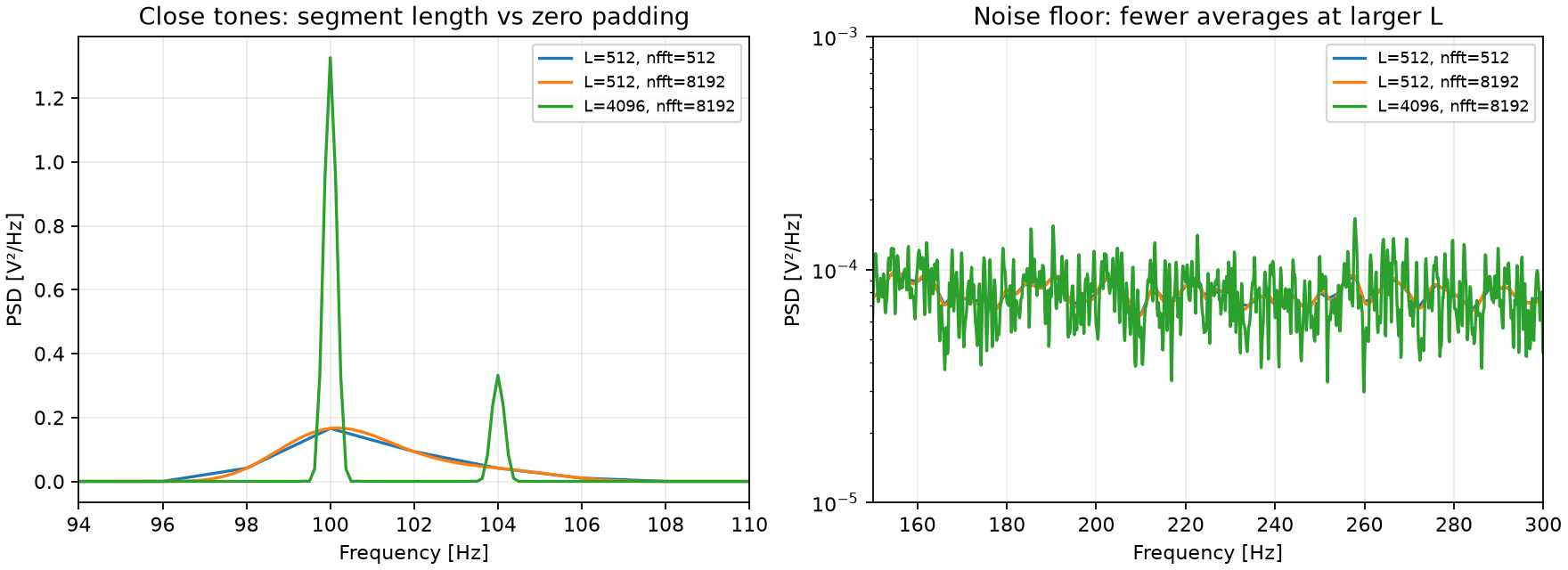
In the left panel, zero padding gives a denser curve for the 512-sample segment, but the broad peaks remain. The 4096-sample segments narrow the window’s frequency response and separate the components. In the right panel, the longer-segment estimate fluctuates more because it has fewer averages. This is one fixed-seed record comparison, not an estimate of confidence intervals.
Integrating PSD: why whole-record variance is not an exact match
The code uses np.sum(p) * df, including both DC and Nyquist bins. For a one-sided PSD of a real signal, the interior bins already include power from corresponding negative frequencies. Do not double them again.
For average='mean', the sum agrees, up to numerical precision, with:
Here \(\widetilde{x}_i\)
is each segment after its own mean has been removed. The second assert verifies this Parseval relation.
In contrast, np.var(x) weights the entire record uniformly. Segment-specific mean removal, window weighting, and how often samples near record boundaries contribute all differ. Sufficiently long segments and appropriate averaging can give a useful approximation, but components with fixed phase relationships can retain differences. Exact equality is not a valid universal requirement.
In this example, the 512-sample integral, 0.744158 V², exceeds the whole-record variance, 0.661787 V². The nearby fixed-phase tones have a cross term that does not vanish under squared-Hann weighting; this hop repeatedly samples the same relative phase. A noise-free control gives 0.708333 V² for 512-sample segments and 0.625000 V² for 4096-sample segments, versus a whole-record variance of 0.625000 V².
Passing the Parseval assert therefore confirms correct normalization of windowed segments, not equally accurate total-power estimation for every segment length. Zero padding does not fix this difference either.
The trapezoidal rule assigns half weights to endpoints, so it differs from this discrete FFT power sum. A large DC component makes the difference particularly visible. Use sum * df for the complete-bin Parseval check; for a selected band, choose an integration convention that explicitly handles boundary bins.
detrend: do you need DC power or fluctuations?
detrend='constant' removes the mean of each segment. Besides DC, this can affect very-low-frequency components with periods longer than a segment. It is not automatically harmless preprocessing for low-frequency measurements.
To examine mean-square power including DC, append:
print(f'variance={np.var(x):.6f} mean_square={np.mean(x**2):.6f}')
w = get_window('hann', 4096, fftbins=True)
f, p = welch(x, fs=fs, window=w, nperseg=4096, noverlap=2048,
             nfft=8192, detrend=False, scaling='density', average='mean')
print(f'no_detrend_power={np.sum(p) * (f[1] - f[0]):.6f}')
Executed output (NumPy 2.5.4, SciPy 1.18.1):
variance=0.661787 mean_square=4.656620
no_detrend_power=4.653860
Mean-square power includes approximately \(2^2=4\)
V² from the offset. Comparing the detrend=False integral with variance and calling the extra 4 V² an error would confuse two different quantities.
A practical workflow for measured data
- Verify
fs, its units, and equal sample spacing. Do not feed irregular timestamps directly into ordinary Welch estimation. - Choose
npersegfrom the peak separation you need and how long the signal remains stationary. - Start with a Hann window and 50% overlap, and calculate the segment count \(K\) .
- Compare
nfft=npersegwith zero padding, keeping grid spacing separate from resolving power. - Check power using the integrated
densityresult; confirm DC treatment, detrending, and input units. - Change the settings by one meaningful step and compare another recording to test whether the conclusion persists.
PSD summarizes time-averaged power by frequency. Choose its parameters together with the decision of whether averaging away transients and time variation is appropriate.
Frequently asked questions
Does increasing nfft improve Welch frequency resolution?
It makes the output frequency grid finer, but does not improve separation of nearby components with unchanged segment length and window. Check nperseg and the window’s frequency width.
Does integrated PSD equal signal variance?
Summing all density bins times the frequency spacing gives the averaged window-weighted segment mean square. With sufficiently long segments and appropriate averaging it can approximate variance, but fixed-phase nearby components can retain a difference. Exact agreement with whole-record variance is not generally valid.
How much overlap should Welch PSD use?
With a Hann window, start at 50%. More overlap produces more segments, but also more correlation; independent averages do not increase at the same rate.
Related articles
- FFT amplitude scaling and zero-padding : one-sided amplitude, window correction, and zero-padding normalization, distinct from PSD.
- Window functions and PSD estimation : frequency responses, leakage, and scalloping.
- DTFT, DFT, and FFT : evaluating the spectrum of finite data.
- Sampling theorem and aliasing : sampling conditions to verify before PSD estimation.
- Choosing a time–frequency analysis method : when a time-averaged PSD is insufficient.