ベイズ最適化の基礎とPython実装

ベイズ最適化とは

ベイズ最適化（Bayesian Optimization）は、評価コストの高いブラックボックス関数の大域的最適化のための手法です。以下のような問題に適しています：

ここで \(f\) は解析的な勾配が得られず、1回の評価に大きなコスト（時間・費用）がかかる関数です。典型的な応用例として、機械学習モデルのハイパーパラメータ最適化、実験計画、材料探索などがあります。

ベイズ最適化は以下の2つの要素で構成されます：

1. 代理モデル（Surrogate Model）: 目的関数を近似する確率モデル（通常はガウス過程）
2. 獲得関数（Acquisition Function）: 次に評価すべき点を決定する関数

少数の観測データから代理モデルを構築し、獲得関数を最大化する点を逐次的に選択することで、効率的に最適解を探索します。

ガウス過程回帰

カーネル関数

ガウス過程（Gaussian Process, GP）は、関数の事前分布を定義する確率モデルです。GPは平均関数 \(m(\mathbf{x})\) とカーネル関数 \(k(\mathbf{x}, \mathbf{x}')\) で特徴付けられます：

最も広く使われるカーネルはRBF（Radial Basis Function）カーネル（二乗指数カーネルとも呼ばれる）です：

ここで \(\sigma_f^2\) は出力の分散、\(l\) は長さスケールパラメータです。\(l\) が大きいほど関数は滑らかになります。

事後分布

\(n\) 個の観測データ \(\mathcal{D} = \{(\mathbf{x}_i, y_i)\}_{i=1}^n\) が与えられたとき、新しい入力 \(\mathbf{x}_*\) での予測分布は以下のようになります。観測ノイズ \(\sigma_n^2\) を仮定すると：

ここで：

• \(\mathbf{K}\) は \(n \times n\) のカーネル行列で \(K_{ij} = k(\mathbf{x}_i, \mathbf{x}_j)\)
• \(\mathbf{k}_* = [k(\mathbf{x}_1, \mathbf{x}_*), \ldots, k(\mathbf{x}_n, \mathbf{x}_*)]^T\)
• \(\mathbf{y} = [y_1, \ldots, y_n]^T\)

式(4)は予測平均、式(5)は予測の不確実性を表します。データが密な領域では \(\sigma^2\) が小さくなり、データが少ない領域では大きくなります。

獲得関数

獲得関数は「次にどこを評価すべきか」を決定します。予測平均（活用）と予測分散（探索）のバランスをとることが重要です。

Expected Improvement（EI）

現在の最良値 \(f(\mathbf{x}^+)\) からの改善量の期待値を最大化します：

ガウス過程の予測分布を用いると、EIは解析的に計算できます：

ここで \(\Phi\) と \(\phi\) はそれぞれ標準正規分布の累積分布関数と確率密度関数、\(\xi \geq 0\) は探索を促進するパラメータです。最小化問題の場合、\(f(\mathbf{x}^+)\) は現在の最小観測値です。

EIの導出（式7・8の証明）

式(6)は期待値のままでは計算できないため、GP事後分布の性質を使って解析的な閉形式に変形します。改善量を

と定義します。GP事後分布より \(f(\mathbf{x}) \sim \mathcal{N}(\mu(\mathbf{x}), \sigma^2(\mathbf{x}))\) なので、\(u\) を \(f(\mathbf{x})\) の実現値とすると期待値は次の積分になります：

ここで \(\varphi\) は平均 \(\mu(\mathbf{x})\) 、分散 \(\sigma^2(\mathbf{x})\) の正規分布の密度関数です。標準化変数 \(z = (u - \mu(\mathbf{x})) / \sigma(\mathbf{x})\) で置換すると、積分上限は \(Z = (f(\mathbf{x}^+) - \mu(\mathbf{x})) / \sigma(\mathbf{x})\) になり：

ここで \(\phi\) は標準正規分布の密度関数です。この積分を2項に分解すると：

第1項の積分は標準正規分布の累積分布関数の定義そのものなので \(\Phi(Z)\) です。第2項は正規分布密度の微分公式 \(\frac{d}{dz}[-\phi(z)] = z \phi(z)\) より原始関数が \(-\phi(z)\) であるとわかるので、

となります（\(z \to -\infty\) で \(\phi(z) \to 0\) であることを使いました）。これらを式(14)へ代入すると：

が得られ、これはまさに式(7)です。探索を促す項 \(\xi \geq 0\) を導入して \(f(\mathbf{x}^+)\) を \(f(\mathbf{x}^+) - \xi\) に置き換えれば式(7)(8)の完全な形になります。\(\xi\) は「現在の最良値をどれだけ上回れば改善とみなすか」の閾値を引き上げる役割を持ち、\(\xi\) を大きくするほどEIは探索寄りになります。

Upper Confidence Bound（UCB）

予測平均から予測標準偏差のスケーリングを引いたものを最小化します（最小化問題の場合はLower Confidence Bound）：

\(\kappa > 0\) は探索と活用のトレードオフを制御します。\(\kappa\) が大きいほど探索的になります。

Probability of Improvement（PI）

現在の最良値を改善する確率を最大化します：

PIは計算が簡単ですが、改善量の大きさを考慮しないため、局所解に収束しやすい欠点があります。

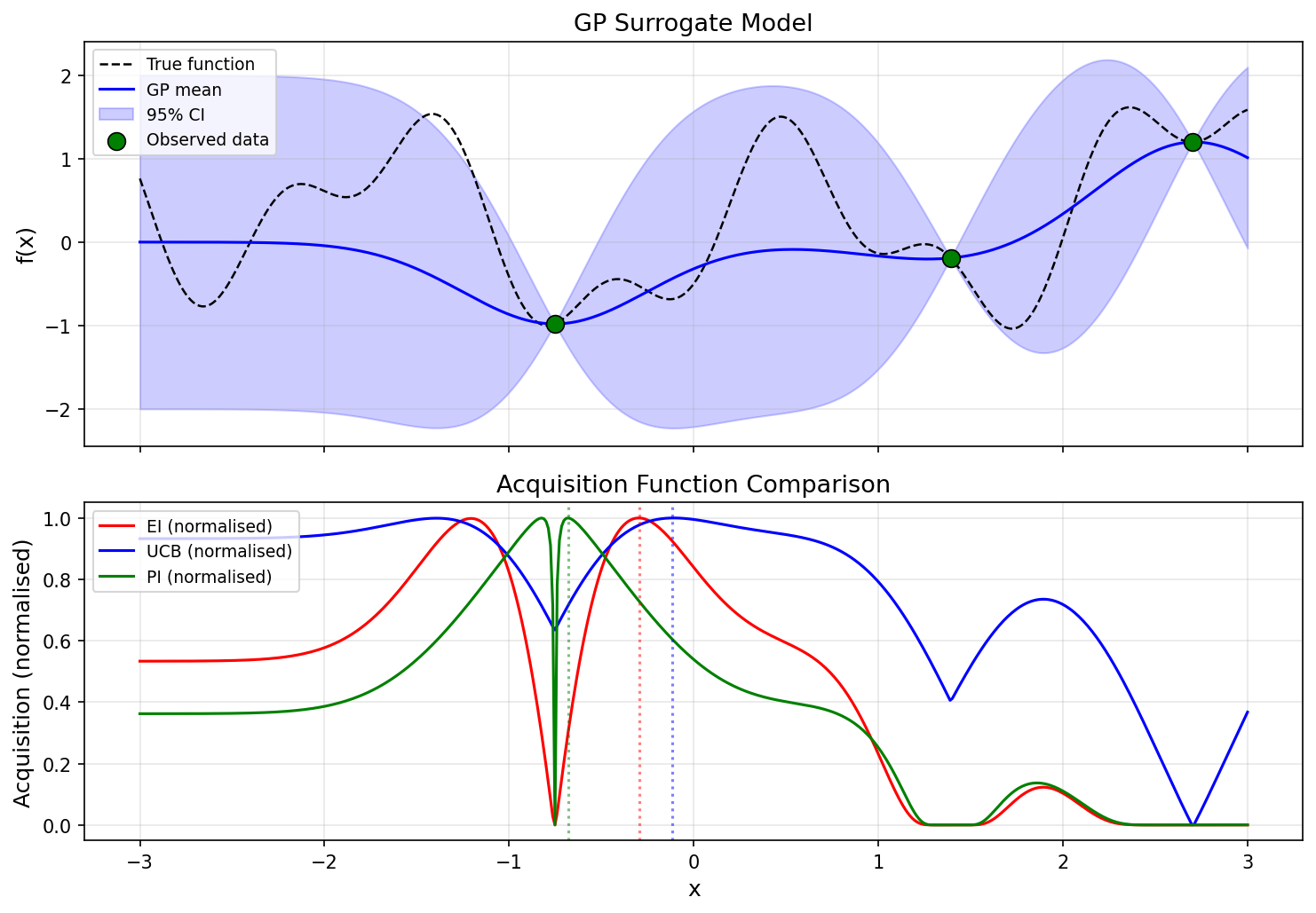
以下の図は、同じGPサロゲートモデルに対して3つの獲得関数がどのように異なる探索戦略を示すかを比較したものです。

Python実装

ガウス過程クラス

NumPyとSciPyを用いてガウス過程回帰をスクラッチで実装します。

import numpy as np
from scipy.stats import norm

class GaussianProcess:
    def __init__(self, length_scale=1.0, signal_var=1.0, noise_var=1e-6):
        self.l = length_scale
        self.sf2 = signal_var
        self.sn2 = noise_var
        self.X_train = None
        self.y_train = None
        self.K_inv = None

    def kernel(self, X1, X2):
        """RBFカーネル（式3）"""
        dist_sq = np.sum(X1**2, axis=1, keepdims=True) \
                  - 2.0 * X1 @ X2.T \
                  + np.sum(X2**2, axis=1)
        return self.sf2 * np.exp(-0.5 * dist_sq / self.l**2)

    def fit(self, X, y):
        """観測データでGPを学習"""
        self.X_train = X.copy()
        self.y_train = y.copy()
        K = self.kernel(X, X) + self.sn2 * np.eye(len(X))
        self.K_inv = np.linalg.inv(K)

    def predict(self, X_new):
        """新しい点での予測平均と予測分散（式4, 5）"""
        k_star = self.kernel(self.X_train, X_new)
        mu = k_star.T @ self.K_inv @ self.y_train
        var = self.sf2 - np.diag(k_star.T @ self.K_inv @ k_star)
        var = np.maximum(var, 1e-10)
        return mu, var

獲得関数の実装

def expected_improvement(mu, var, y_best, xi=0.01):
    """Expected Improvement（式7, 8）"""
    sigma = np.sqrt(var)
    with np.errstate(divide="ignore", invalid="ignore"):
        Z = (y_best - mu - xi) / sigma
        ei = (y_best - mu - xi) * norm.cdf(Z) + sigma * norm.pdf(Z)
        ei[sigma < 1e-10] = 0.0
    return ei

def upper_confidence_bound(mu, var, kappa=2.0):
    """UCB（最小化用：LCB）（式9）"""
    sigma = np.sqrt(var)
    return mu - kappa * sigma

def probability_of_improvement(mu, var, y_best, xi=0.01):
    """Probability of Improvement（式10）"""
    sigma = np.sqrt(var)
    with np.errstate(divide="ignore", invalid="ignore"):
        Z = (y_best - mu - xi) / sigma
        pi = norm.cdf(Z)
        pi[sigma < 1e-10] = 0.0
    return pi

ベイズ最適化ループ

def bayesian_optimization(f, bounds, n_init=3, n_iter=15,
                          acq_func="ei"):
    """ベイズ最適化のメインループ"""
    # 初期点のランダムサンプリング
    X_init = np.random.uniform(bounds[0], bounds[1],
                               size=(n_init, 1))
    y_init = np.array([f(x) for x in X_init]).reshape(-1)

    gp = GaussianProcess(length_scale=0.5, signal_var=1.0,
                         noise_var=1e-6)
    X_sample = X_init.copy()
    y_sample = y_init.copy()

    # 最適化ループ
    for i in range(n_iter):
        gp.fit(X_sample, y_sample)

        # 候補点での獲得関数の評価
        X_cand = np.linspace(bounds[0], bounds[1], 500).reshape(-1, 1)
        mu, var = gp.predict(X_cand)
        y_best = np.min(y_sample)

        if acq_func == "ei":
            acq = expected_improvement(mu, var, y_best)
            x_next = X_cand[np.argmax(acq)]
        elif acq_func == "ucb":
            acq = upper_confidence_bound(mu, var)
            x_next = X_cand[np.argmin(acq)]
        elif acq_func == "pi":
            acq = probability_of_improvement(mu, var, y_best)
            x_next = X_cand[np.argmax(acq)]

        # 新しい点を評価して追加
        y_next = f(x_next.reshape(1, -1))
        X_sample = np.vstack([X_sample, x_next.reshape(1, -1)])
        y_sample = np.append(y_sample, y_next)

    return X_sample, y_sample, gp

1D最適化デモ

テスト関数としてノイズのない非凸関数を使い、ベイズ最適化の挙動を確認します。

import matplotlib.pyplot as plt

def test_function(x):
    """複数の極小値を持つテスト関数"""
    return np.sin(3 * x) + x**2 * 0.1 - 0.5 * np.cos(7 * x)

np.random.seed(42)
bounds = (-3.0, 3.0)
X_sample, y_sample, gp = bayesian_optimization(
    test_function, bounds, n_init=3, n_iter=12, acq_func="ei"
)

# 最適化結果のプロット
X_plot = np.linspace(bounds[0], bounds[1], 300).reshape(-1, 1)
y_true = np.array([test_function(x) for x in X_plot])
mu, var = gp.predict(X_plot)
sigma = np.sqrt(var)

fig, axes = plt.subplots(2, 1, figsize=(10, 8))

# GP代理モデル
axes[0].plot(X_plot, y_true, "k--", label="True function")
axes[0].plot(X_plot, mu, "b-", label="GP mean")
axes[0].fill_between(X_plot.ravel(), mu - 2*sigma, mu + 2*sigma,
                     alpha=0.2, color="blue", label="95% CI")
axes[0].scatter(X_sample[:3], y_sample[:3],
                c="green", s=80, zorder=5, label="Initial points")
axes[0].scatter(X_sample[3:], y_sample[3:],
                c="red", s=80, zorder=5, label="BO samples")
axes[0].set_xlabel("x")
axes[0].set_ylabel("f(x)")
axes[0].set_title("Bayesian Optimization with GP Surrogate")
axes[0].legend()
axes[0].grid(True)

# EI獲得関数
acq_ei = expected_improvement(mu, var, np.min(y_sample))
axes[1].plot(X_plot, acq_ei, "r-", label="EI")
axes[1].set_xlabel("x")
axes[1].set_ylabel("EI(x)")
axes[1].set_title("Expected Improvement")
axes[1].legend()
axes[1].grid(True)

plt.tight_layout()
plt.savefig("bayesian_optimization_result.png", dpi=150)
plt.show()

best_idx = np.argmin(y_sample)
print(f"Best x: {X_sample[best_idx].item():.4f}")
print(f"Best f(x): {y_sample[best_idx]:.4f}")
print(f"Total evaluations: {len(y_sample)}")

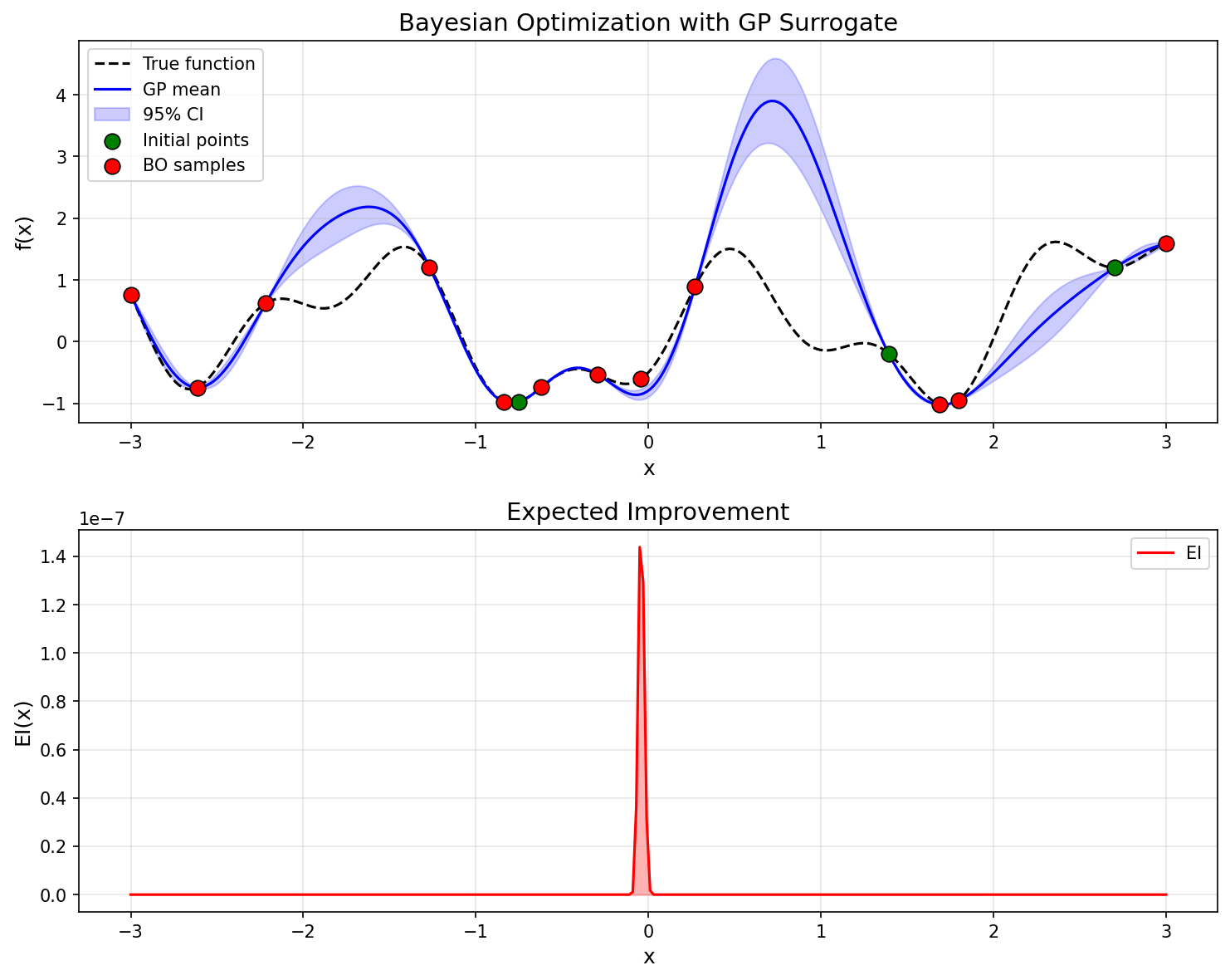
GPの予測平均（青線）が真の関数（黒点線）に近づいていく様子と、信頼区間（青い帯）がデータ付近で狭くなる様子が確認できます。EIは不確実性が高く改善が期待される領域で大きな値をとり、探索と活用のバランスを自動的に調整します。

実行結果

上記のコードを実際に実行しました（numpy 2.4.2、scipy 1.18.0、matplotlib 3.10.8 で検証済み）。EI獲得関数を使った最適化ループの出力は次の通りです：

Best x: 1.6894
Best f(x): -1.0210
Total evaluations: 15

テスト関数の真の大域最小値は、2,000,001点の高密度格子探索により \(\mathbf{x}^* = 1.723911\) 、\(f(\mathbf{x}^*) = -1.038189\) と特定できます（この全数探索的な答え合わせは、評価コストが安い検証専用の計算であり、実務のブラックボックス最適化では利用できないことに注意してください）。したがって、EIによる15回の評価（初期点3 + ループ12回）で得られた解の残差（regret）は \(\lvert -1.0210 - (-1.038189) \rvert \approx 0.0172\) でした。

同一シード・同一初期点で acq_func="ucb" と acq_func="pi" に切り替えて実行した結果も含めてまとめます：

下図はイテレーションごとの「これまでの最良値（best-so-far）」の推移を3手法で比較したものです。

この特定の実行では PI が最も速く・最も真の最適値に近い解に収束していますが、後述するようにこれは単一シードの結果に過ぎず一般化できません。PIは改善確率のみを最大化し改善量の大きさを無視するため、一度良い局所解を見つけると強く活用（exploit）する傾向があり、たまたま今回のテスト関数・シードの組み合わせで有利に働いただけです。多数の目的関数・シードにわたる平均的な性能では、改善量の大きさを考慮するEIと、理論的なregret保証を持つUCBの方が頑健な選択とされています（Shahriari et al., 2016）。

実践上の注意点とエッジケース

教科書的な定式化をそのままコードにする際に見落としがちな落とし穴を整理します。

1. \(\sigma(\mathbf{x}) \to 0\) における数値的特異点

観測済みの点やその近傍では予測分散 \(\sigma^2(\mathbf{x})\) がほぼ0になります。式(8)の \(Z\) はゼロ除算になり、素朴に実装するとNaN/Infが発生します。本記事のコードでは np.errstate でゼロ除算警告を抑制した上で ei[sigma < 1e-10] = 0.0 により明示的にマスクしています。これは「不確実性がない点では追加の改善余地はない」という数学的に正しい極限（\(\sigma \to 0^+\) で \(\text{EI} \to 0\) ）に対応しており、マスク処理を忘れると獲得関数の最大化で誤ってNaNを選んでしまうバグになります。

2. カーネル行列の悪条件化

GaussianProcess.fit は np.linalg.inv(K) で愚直に逆行列を計算していますが、観測点が近接すると \(\mathbf{K}\) の条件数が急激に悪化し、逆行列計算が数値的に不安定になります（浮動小数点誤差で予測分散が負になることすらあります）。実運用ライブラリ（scikit-learnのGaussianProcessRegressorなど）はCholesky分解（scipy.linalg.cho_factor / cho_solve）を使い、逆行列を明示的に計算しない方が数値的に安定です。本記事のスクラッチ実装は教育目的で単純化していることに注意してください（Choleskyベースの実装は ガウス過程回帰の実践 で解説しています）。

3. \(\xi\) （EI/PI）と \(\kappa\) （UCB）のスケール依存性

\(\xi\) は \(f(\mathbf{x})\) のスケールに対して絶対値で効くパラメータです。目的関数の値域が変われば適切な \(\xi\) も変わるため、実務では観測値の標準偏差でスケーリングする（例：\(\xi = 0.01 \times \text{std}(y)\) ）方が安全です。\(\kappa\) についても、GP-UCBの理論的なregret保証は反復回数 \(t\) に応じたスケジューリングを要求します：

（\(d\) は入力次元、\(\delta\) は失敗確率。Srinivas et al., 2010）。本記事のデモでは固定値 \(\kappa=2\) を使いましたが、これは反復回数が少ない実務でよく使われる簡略化であり、理論的なno-regret保証は保持しません。

4. 単一シードの結果を一般化しない

前節で見た通り、EI・UCB・PIを同一のシード（seed=42）・同一の初期点で12回実行した結果、PIが最も良い値に到達しました。しかし、ある1回の実行でPIが優れていたからといって「PIの方が優れている」と結論づけるのは誤りです。統計的に妥当な比較には複数シードでの反復・平均、および複数のテスト関数（多峰性・次元数を変えたベンチマーク）が必須です。

5. 獲得関数最適化自体の非凸性

本実装では候補点を np.linspace で500点の格子上に固定し、その中で argmax を取ることで獲得関数を「最適化」しています。これは1次元だから許容できる近似であり、次元 \(d\) が増えると必要な格子点数が指数的に爆発します（次元の呪い）。実務のBOライブラリ（scipy.optimize.minimize によるマルチスタートL-BFGS-Bなど）は獲得関数自体の非凸最適化を勾配法で解きますが、獲得関数も局所最適に収束しうるため複数の初期値からの再スタートが必要です。

6. ガウス過程のスケーラビリティと適用限界

式(4)(5)の \((\mathbf{K} + \sigma_n^2\mathbf{I})^{-1}\) の計算コストは \(O(n^3)\) （\(n\) は観測点数）であり、数百〜数千回の評価を超えると実用的でなくなります。またBOが効果的なのはおおむね20次元程度までで、それ以上では獲得関数最適化の難化とカーネルのスパース性の欠如により性能が劣化します（Shahriari et al., 2016）。

7. ノイズ分散とカーネルハイパーパラメータの手動固定

本実装では length_scale=0.5、noise_var=1e-6 を手動で固定しています。実際のハイパーパラメータ最適化のように目的関数の評価にノイズが乗る場合（例：確率的勾配降下法で学習したモデルの検証精度は乱数シードで変動する）、noise_var を0に近い値に固定すると過学習的にノイズを追いかけてしまいます。実務では対数周辺尤度最大化でこれらのハイパーパラメータ自体を学習する必要があります（詳細は ガウス過程回帰の実践 を参照）。

8. 発展的な研究動向：LLMを用いた高度化

近年、大規模言語モデル（LLM）をベイズ最適化のコンポーネントとして組み込む研究が進んでいます。Liu et al. (2024) の LLAMBO（“Large Language Models to Enhance Bayesian Optimization”、ICLR 2024）は、最適化問題を自然言語で記述しLLMに文脈内学習（few-shot learning）させることで、観測履歴が少ない探索初期段階でのサロゲートモデルの性能を補強する手法を提案しています。ファインチューニングを必要とせず、観測がまばらな探索初期で特に有効であり、多様なハイパーパラメータチューニングのベンチマークで強い性能を示すことが報告されています。本記事で解説したEI/UCB/PIのようなガウス過程ベースの獲得関数は依然として標準的な基盤ですが、LLMを外部知識源として組み合わせるハイブリッドなアプローチは今後の発展が期待される方向性です。

CEM・MPPIとの比較

ベイズ最適化は クロスエントロピー法（CEM） や MPPI とは異なるアプローチの最適化手法です。以下に比較をまとめます。

• ベイズ最適化は1回の評価が高コストな場合に最適です。代理モデルにより少ない評価回数で効率的に探索しますが、ガウス過程の計算コストにより高次元への適用が難しくなります。
• CEMはサンプルベースの手法で、多数の評価が可能な場合に有効です。エリートサンプルのハードな選択により分布を更新します。
• MPPIはCEMと同様にサンプルベースですが、ソフトな重み付けにより全サンプルの情報を活用します。リアルタイムの制御問題に適しています。

おすすめ書籍

ガウス過程の理論からベイズ最適化への応用まで、日本語で体系的に学べる決定版です。

ベイズ推論の枠組みをゼロから積み上げる入門書で、本記事の背後にある確率モデリングの考え方を補強できます。

※ 上記は Amazon アソシエイトのリンクです。

関連記事

• 焼きなまし法（Simulated Annealing）の理論とPython実装 - 温度パラメータによる確率的探索を行うメタヒューリスティクスを解説しています。
• 遺伝的アルゴリズム（GA）の理論とPython実装 - 進化的計算に基づくブラックボックス最適化手法を解説しています。
• 確率的勾配降下法からAdamまで - 勾配ベースの最適化手法。ベイズ最適化はハイパーパラメータチューニングに使われます。
• MCMC入門：メトロポリス・ヘイスティングス法とギブスサンプリング - ベイズ最適化の背景にあるベイズ推論の計算手法を解説しています。
• Hamiltonian Monte Carlo（HMC）の理論とPython実装 - GPハイパーパラメータの完全ベイズ推定など、獲得関数計算の背後で高相関事後分布を効率的にサンプリングする手法として関連します。
• 粒子群最適化（PSO）の数理とPython実装 - 群知能ベースのメタヒューリスティクス。評価コストが安い問題で速度を優先するPSOと、評価コストが高い問題に強いベイズ最適化の使い分けを比較できます。
• ガウス過程回帰の理論とPython実装 - ベイズ最適化のサロゲートモデル本体。本記事のEI/UCB/PIがGPの予測平均と分散から構成されることを確認できます。
• ガウス過程回帰の実践：カーネル設計と応用 - サロゲートモデルの質を左右するカーネル設計の実践編。カーネルの選択・合成がベイズ最適化の探索性能に直結します。
• モンテカルロ最適化メソッド比較（CEM/SA/GA/MPPI/PSO） - サンプリングベースの最適化手法（CEM/SA/GA/MPPI/PSO）を「サンプリング→評価→更新」の共通骨格で比較するハブ記事。評価コストが高い問題向けのベイズ最適化との使い分けが整理できます。
• 機械学習による時系列予測・分類・異常検知ハブ - ベイズ最適化を GBDT・LSTM・GMM のハイパパラ自動探索シナリオに位置づけ、機械学習全体地図の中で「ハイパパラ最適化レイヤ」として組み込み方を示すハブ記事。
• アンサンブル学習（Random Forest / Gradient Boosting） - learning_rate / num_leaves / max_depth / n_estimators の組み合わせ探索は典型的なベイズ最適化案件。TPE が標準的に強い領域です。
• LSTMによる時系列予測のPython実装 - hidden_size / layers / lookback / dropout / learning_rate を GP-EI で 30 試行程度に圧縮できる代表例。長時間の学習を伴うため評価コスト型の典型問題です。

参考文献

• Rasmussen, C. E., & Williams, C. K. I. (2006). Gaussian Processes for Machine Learning. MIT Press.
• Shahriari, B., et al. (2016). “Taking the Human Out of the Loop: A Review of Bayesian Optimization.” Proceedings of the IEEE, 104(1), 148-175.
• Snoek, J., Larochelle, H., & Adams, R. P. (2012). “Practical Bayesian Optimization of Machine Learning Algorithms.” NeurIPS 2012.
• Brochu, E., Cora, V. M., & de Freitas, N. (2010). “A Tutorial on Bayesian Optimization of Expensive Cost Functions.” arXiv:1012.2599.
• Srinivas, N., Krause, A., Kakade, S. M., & Seeger, M. (2010). “Gaussian Process Optimization in the Bandit Setting: No Regret and Experimental Design.” ICML 2010.
• Liu, T., Astorga, N., Seedat, N., & van der Schaar, M. (2024). “Large Language Models to Enhance Bayesian Optimization.” ICLR 2024. arXiv:2402.03921.