粒子フィルタのPython実装：リサンプリング手法の比較

粒子フィルタとは

粒子フィルタ（パーティクルフィルタ）は、逐次モンテカルロ法（Sequential Monte Carlo, SMC）に基づく非線形フィルタリング手法です。状態の事後分布を多数の重み付きサンプル（粒子）で近似することで、ガウス分布の仮定を必要とせず、任意の非線形・非ガウスシステムに適用できます。

Cubature Kalman Filter（CKF） や、 Unscented変換（U変換） に基づく Unscented Kalman Filter（UKF）はガウス近似に基づくため、事後分布が多峰性を持つ場合や強い非線形性がある場合には推定精度が低下します。粒子フィルタはこのような場合にも有効な手段です。

粒子フィルタは クロスエントロピー法（CEM） と同じくモンテカルロサンプリングを基盤とする手法ですが、CEMが最適化問題を対象とするのに対し、粒子フィルタは時系列の状態推定を対象とします。

アルゴリズムの概要

状態空間モデル

以下の非線形状態空間モデルを考えます：

ここで \(f\) は状態遷移関数、\(h\) は観測関数、\(w_{k-1}\) と \(v_k\) はそれぞれプロセスノイズと観測ノイズです。ノイズ分布 \(p_w, p_v\) はガウス分布である必要はありません。

逐次モンテカルロの枠組み

粒子フィルタは \(N\) 個の粒子 \(\{x_k^{(i)}, w_k^{(i)}\}_{i=1}^{N}\) で事後分布 \(p(x_k | y_{1:k})\) を近似します。各ステップは以下の3つのフェーズからなります。

1. 予測（Prediction）： 各粒子を状態遷移モデルに従って伝播させます：

実装上は、\(x_k^{(i)} = f(x_{k-1}^{(i)}) + w_{k-1}^{(i)}\) としてプロセスノイズを加えます。

2. 重み更新（Weight Update）： 新しい観測 \(y_k\) に基づき、各粒子の尤度を計算して重みを更新します：

3. 正規化（Normalization）： 重みの総和が1になるように正規化します：

正規化された重みを用いて、状態の推定値は以下で計算されます：

重要度サンプリングからの導出

前節の重み更新式 \(w_k^{(i)} \propto p(y_k \mid x_k^{(i)})\) は天下り的に見えますが、これは**逐次重要度サンプリング（Sequential Importance Sampling, SIS）**の一般式を、特定の提案分布（proposal distribution）に対して簡略化したものです。ここでは一般式からの導出を示します。

重要度サンプリングの原理

目標分布 \(p(x_{0:k} \mid y_{1:k})\) から直接サンプリングできない場合、提案分布 \(q(x_{0:k} \mid y_{1:k})\) から粒子 \(x_{0:k}^{(i)} \sim q\) を生成し、以下の重要度重みで補正します：

このとき、任意の関数 \(g\) の期待値は自己正規化重要度サンプリング（self-normalized importance sampling）推定量

で近似できます。問題は、時刻 \(k\) が進むごとに軌跡全体 \(x_{0:k}\) の次元が増加し、重みを毎回ゼロから計算し直すと計算量が時間とともに発散することです。

逐次計算への分解

提案分布をマルコフ的に分解します：

目標分布側も、状態空間モデルのマルコフ性とベイズの定理から

と分解できます（証明：\(p(x_{0:k}, y_{1:k}) = p(x_0) \prod_t p(x_t \mid x_{t-1}) p(y_t \mid x_t)\) は状態空間モデルの生成過程そのものであり、\(p(x_{0:k} \mid y_{1:k}) \propto p(x_{0:k}, y_{1:k})\) から従います）。

両者の比を取ると、重みは時刻 \(k-1\) の重みに、時刻 \(k\) の新しい因子だけを掛けた逐次更新式になります：

これが逐次重要度サンプリングの一般式です。\(x_{0:k-1}\) 全体を保持しなくても、直前の重み \(w_{k-1}^{(i)}\) と新しい粒子 \(x_k^{(i)}\) だけから更新できる点が、逐次計算を可能にしています。

ブートストラップフィルタとしての特殊化

提案分布として状態遷移モデルそのもの \(q(x_k \mid x_{k-1}, y_k) = p(x_k \mid x_{k-1})\) を選ぶと（つまり観測 \(y_k\) を無視して粒子を伝播させると）、分母と分子の \(p(x_k \mid x_{k-1})\) が打ち消し合い、更新式は

まで単純化されます。リサンプリング直後は \(w_{k-1}^{(i)} = 1/N\) （全粒子が等しい重みを持つ）なので、これは前節の式 \(w_k^{(i)} \propto p(y_k \mid x_k^{(i)})\) と一致します。この特殊化は**ブートストラップフィルタ（bootstrap filter, Gordon, Salmond & Smith, 1993）**と呼ばれ、実装が最も単純である一方、提案分布が観測情報を一切使わないため、尤度 \(p(y_k \mid x_k)\) が鋭く尖っている（観測ノイズが小さい）場合には重みの分散が大きくなりやすいという欠点を持ちます。本記事のコード実装はこのブートストラップフィルタです。

有効サンプルサイズと縮退

粒子フィルタの大きな課題は**重みの縮退（weight degeneracy）**です。時間が経過するにつれて、ほとんどの粒子の重みが0に近づき、少数の粒子だけが大きな重みを持つようになります。

この縮退の度合いを定量化するのが**有効サンプルサイズ（Effective Sample Size, ESS）**です：

\(N_{\text{eff}}\) は1から \(N\) の値をとり、すべての重みが等しい場合（縮退なし）に \(N\) となります。\(N_{\text{eff}}\) が閾値（例えば \(N/2\) ）を下回ったときにリサンプリングを実行することで、縮退を緩和します。

有効サンプルサイズの導出

上記の式も天下り的に見えますが、Kong, Liu & Wong (1994) による近似から導出できます。理想的には、目標分布から直接 \(N\) 個の独立同分布サンプルを得られたときの推定量の分散を基準に、自己正規化重要度サンプリング推定量の分散が何倍に劣化するかを測りたいところです。彼らは、この劣化係数が、正規化前の重み比 \(r^{(i)} = p(x^{(i)})/q(x^{(i)})\) の変動係数（coefficient of variation）の2乗

を用いて \(1 + \mathrm{CV}^2(w)\) と近似できることを示しました。したがって、有効サンプルサイズは

と定義されます。ここで正規化された重み \(\tilde{w}^{(i)}\) （\(\sum_i \tilde{w}^{(i)} = 1\) ）を使うと、その標本平均は \(1/N\) なので、\(\mathrm{CV}^2(w)\) は次のように書き換えられます：

（展開の際に \(\sum_i \tilde{w}^{(i)} = 1\) を用いました）。これを \(N_{\text{eff}}\) の式に代入すると

となり、コードで用いている式が導かれます。全粒子の重みが等しい（\(\tilde{w}^{(i)} = 1/N\) ）とき \(\mathrm{CV}^2 = 0\) で \(N_{\text{eff}} = N\) 、逆に1粒子に重みが集中する（他は0）とき \(\mathrm{CV}^2 \to N-1\) で \(N_{\text{eff}} \to 1\) となり、直感と整合します。

def effective_sample_size(weights):
    """有効サンプルサイズの計算"""
    return 1.0 / np.sum(weights ** 2)

リサンプリングがなぜ必要か：重みの分散増大の証明

前節の重み更新式 \(w_k^{(i)} \propto w_{k-1}^{(i)} \cdot p(y_k \mid x_k^{(i)}) p(x_k^{(i)} \mid x_{k-1}^{(i)}) / q(\cdot)\) は乗算的な漸化式です。各時刻で新たに掛かる因子が粒子ごとにばらつきを持つ限り（提案分布 \(q\) が目標分布と厳密に一致しない限り、これは一般に成り立ちます）、重みの対数 \(\log w_k^{(i)}\) は、独立な確率変動を毎時刻加算していくランダムウォークになります。したがって \(\mathrm{Var}(w_k)\) は時間について単調非減少であり、リサンプリングを行わない限り \(k \to \infty\) で重みの分散は発散し、\(N_{\text{eff}} \to 1\) に収束することが示されています（Doucet, Godsill & Andrieu, 2000）。リサンプリングは、\(N_{\text{eff}}\) が閾値を下回った時点で重みをいったん均等化することで、このランダムウォークを定期的にリセットし、分散の発散を防ぐ役割を持ちます。これが「リサンプリングがなぜ必要か」に対する形式的な根拠です。

リサンプリング手法

リサンプリングでは、重みの大きい粒子を複製し、重みの小さい粒子を除去することで、粒子集合を再構成します。以下に3つの代表的な手法と、その比較対象となるベースラインを紹介します。

系統的リサンプリング（Systematic Resampling）

系統的リサンプリングは、一つの乱数 \(u_0\) を生成し、等間隔に配置された点で累積分布関数（CDF）をサンプリングします。計算量が \(O(N)\) で、分散が小さいため実用上最もよく使われます。

def systematic_resampling(weights):
    """系統的リサンプリング"""
    N = len(weights)
    positions = (np.random.random() + np.arange(N)) / N
    cumsum = np.cumsum(weights)
    indices = np.zeros(N, dtype=int)
    i, j = 0, 0
    while i < N:
        if positions[i] < cumsum[j]:
            indices[i] = j
            i += 1
        else:
            j += 1
    return indices

残差リサンプリング（Residual Resampling）

残差リサンプリングは、まず各粒子を \(\lfloor N \tilde{w}^{(i)} \rfloor\) 回確定的に複製し、残りの粒子数を残差重みに基づいて確率的にサンプリングします。確定的な複製が含まれるため、純粋にランダムなサンプリングよりも分散が小さくなります。

def residual_resampling(weights):
    """残差リサンプリング"""
    N = len(weights)
    indices = []

    # 確定的な複製
    num_copies = (N * weights).astype(int)
    for i in range(N):
        indices.extend([i] * num_copies[i])

    # 残差の処理
    residual_weights = N * weights - num_copies
    residual_weights /= residual_weights.sum()
    num_remaining = N - len(indices)
    if num_remaining > 0:
        cumsum = np.cumsum(residual_weights)
        # 残差部分に系統的リサンプリングを適用
        positions = (np.random.random() + np.arange(num_remaining)) / num_remaining
        i, j = 0, 0
        while i < num_remaining:
            if positions[i] < cumsum[j]:
                indices.append(j)
                i += 1
            else:
                j += 1

    return np.array(indices)

層化リサンプリング（Stratified Resampling）

層化リサンプリングは、\([0, 1)\) 区間を \(N\) 等分し、各区間内で独立に一様乱数を生成してCDFをサンプリングします。系統的リサンプリングと似ていますが、各区間で独立な乱数を使う点が異なります。

def stratified_resampling(weights):
    """層化リサンプリング"""
    N = len(weights)
    positions = (np.random.random(N) + np.arange(N)) / N
    cumsum = np.cumsum(weights)
    indices = np.zeros(N, dtype=int)
    i, j = 0, 0
    while i < N:
        if positions[i] < cumsum[j]:
            indices[i] = j
            i += 1
        else:
            j += 1
    return indices

多項リサンプリング（ベースライン）とオフスプリング分散の理論

上記3手法の分散低減効果を定量的に評価するには、比較対象となるベースラインが必要です。**多項リサンプリング（multinomial resampling）**は、正規化重みを確率とするカテゴリカル分布から \(N\) 個の添字を独立に \(N\) 回抽出する、最も素朴な方法です。

def multinomial_resampling(weights):
    """多項リサンプリング（素朴なベースライン）"""
    N = len(weights)
    return np.random.choice(N, size=N, replace=True, p=weights)

オフスプリング数の分散の導出： 粒子 \(i\) が何回複製されるか（オフスプリング数 \(N_i\) 、\(\sum_i N_i = N\) ）を考えます。どのリサンプリング手法でも不偏性 \(\mathbb{E}[N_i] = N \tilde{w}^{(i)}\) は満たされますが、\(\mathrm{Var}(N_i)\) は手法によって大きく異なります。

多項リサンプリングでは、\(N\) 回の独立試行のうち粒子 \(i\) が選ばれる回数なので \(N_i \sim \mathrm{Binomial}(N, \tilde{w}^{(i)})\) に従い、

となります。これは \(\tilde{w}^{(i)} = 1/2\) で最大値 \(N/4\) を取り、\(N\) に比例して増大しえます。

対照的に、系統的・層化リサンプリングでは、CDF上に等間隔（または層化された）位置を置くため、粒子 \(i\) の累積区間（幅 \(\tilde{w}^{(i)}\) ）に含まれる位置の数は \(\lfloor N \tilde{w}^{(i)} \rfloor\) か \(\lceil N \tilde{w}^{(i)} \rceil\) の隣接する2値のいずれかしか取り得ません。2値しか取らない確率変数の分散は最大でも \(1/4\) （ベルヌーイ分布の分散の上界）であるため、

が \(\tilde{w}^{(i)}\) の値によらず成り立ちます。多項リサンプリングの \(N \tilde{w}^{(i)}(1-\tilde{w}^{(i)})\) が \(N\) とともに増大しえるのとは対照的に、こちらは \(N\) に依存しない定数で抑えられます（Douc & Cappe, 2005）。残差リサンプリングは、整数部分を決定的に複製したうえで残差部分にのみ系統的リサンプリングを適用するため、その分散は系統的リサンプリングとほぼ同水準になります。

実測による検証： 歪んだ重みベクトル（\(N=200\) 、指数分布の2乗からサンプル）に対して4手法を2万回ずつ試行し、各粒子のオフスプリング数の分散を実測しました。

np.random.seed(0)
N = 200
raw = np.random.exponential(scale=1.0, size=N) ** 2
weights_fixed = raw / raw.sum()

n_trials = 20000
for name, fn in resamplers.items():
    counts = np.zeros((n_trials, N))
    for t in range(n_trials):
        idx = fn(weights_fixed)
        counts[t] = np.bincount(idx, minlength=N)
    print(f"{name}: mean Var(N_i)={counts.var(axis=0).mean():.4f}, "
          f"max Var(N_i)={counts.var(axis=0).max():.4f}")

結果は理論値と高精度で一致しました：

理論値（二項分布分散の平均 0.9692、最大 21.0006）と実測値はほぼ完全に一致し、系統的・残差リサンプリングの実測最大値（0.2499、0.2498）も理論上界の \(1/4 = 0.25\) と整合します。系統的・残差リサンプリングの合計分散は多項リサンプリングのわずか13.7%であり、Douc & Cappe (2005) が理論的に示した分散低減効果を数値的に裏付けています。層化リサンプリングは各層で独立な乱数を1つずつ（計 \(N\) 個）使うため、系統的リサンプリング（乱数1個のみ）よりランダム性の入力源が多く、分散もやや高くなります（19.5%）。

非線形システムでのデモ

ベンチマークモデル

粒子フィルタの性能を評価するために、広く使われている一変量非定常成長モデル（Univariate Nonstationary Growth Model）を使用します。このモデルは強い非線形性を持ち、ガウス近似に基づくフィルタでは対応が困難です。

状態遷移モデル：

観測モデル：

このモデルの特徴は、観測関数 \(h(x) = x^2/20\) が偶関数であるため、正と負の状態値を区別できず、事後分布が双峰性を持つことがある点です。

粒子フィルタの実装

import numpy as np
import matplotlib.pyplot as plt

# ---- モデルの定義 ----
sigma_w = np.sqrt(10.0)  # プロセスノイズの標準偏差
sigma_v = np.sqrt(1.0)   # 観測ノイズの標準偏差

def state_transition(x, k):
    """状態遷移関数"""
    return x / 2.0 + 25.0 * x / (1.0 + x ** 2) + 8.0 * np.cos(1.2 * k)

def observation(x):
    """観測関数"""
    return x ** 2 / 20.0

def log_likelihood(y, x):
    """対数尤度 log p(y|x)"""
    diff = y - observation(x)
    return -0.5 * (diff ** 2) / (sigma_v ** 2)

# ---- 粒子フィルタ本体 ----
def particle_filter(y_obs, N_particles, resample_fn, resample_threshold=0.5):
    """
    粒子フィルタの実行

    Parameters
    ----------
    y_obs : array, 観測値の系列
    N_particles : int, 粒子数
    resample_fn : callable, リサンプリング関数
    resample_threshold : float, ESS閾値（N_particlesに対する比率）

    Returns
    -------
    x_est : array, 状態推定値の系列
    ess_history : array, ESSの履歴
    """
    T = len(y_obs)
    threshold = resample_threshold * N_particles

    # 初期化：事前分布からサンプリング
    particles = np.random.normal(0, np.sqrt(5.0), N_particles)
    weights = np.ones(N_particles) / N_particles

    x_est = np.zeros(T)
    ess_history = np.zeros(T)

    for k in range(T):
        # 予測：状態遷移 + プロセスノイズ
        particles = state_transition(particles, k + 1) \
                    + sigma_w * np.random.randn(N_particles)

        # 重み更新：対数尤度で計算し、オーバーフローを防ぐ
        log_w = log_likelihood(y_obs[k], particles)
        log_w -= np.max(log_w)  # 数値安定化
        weights = np.exp(log_w)
        weights /= np.sum(weights)

        # 状態推定
        x_est[k] = np.sum(weights * particles)

        # ESS計算
        ess = effective_sample_size(weights)
        ess_history[k] = ess

        # リサンプリング（ESS閾値ベース）
        if ess < threshold:
            indices = resample_fn(weights)
            particles = particles[indices]
            weights = np.ones(N_particles) / N_particles

    return x_est, ess_history

シミュレーションの実行

np.random.seed(42)
T = 100           # タイムステップ数
N_particles = 500  # 粒子数

# 真の状態と観測の生成
x_true = np.zeros(T)
y_obs = np.zeros(T)
x_true[0] = 0.1  # 初期状態

for k in range(1, T):
    x_true[k] = state_transition(x_true[k - 1], k) \
                + sigma_w * np.random.randn()

for k in range(T):
    y_obs[k] = observation(x_true[k]) + sigma_v * np.random.randn()

# 3種類のリサンプリング手法 + 比較用ベースライン（多項）で粒子フィルタを実行
resamplers = {
    "Systematic": systematic_resampling,
    "Residual": residual_resampling,
    "Stratified": stratified_resampling,
    "Multinomial": multinomial_resampling,
}

results = {}
for name, fn in resamplers.items():
    np.random.seed(42)  # 公平な比較のため乱数シードを統一
    x_est, ess_hist = particle_filter(y_obs, N_particles, fn)
    rmse = np.sqrt(np.mean((x_true - x_est) ** 2))
    results[name] = {"estimate": x_est, "ess": ess_hist, "rmse": rmse}
    print(f"{name}: RMSE = {rmse:.4f}")

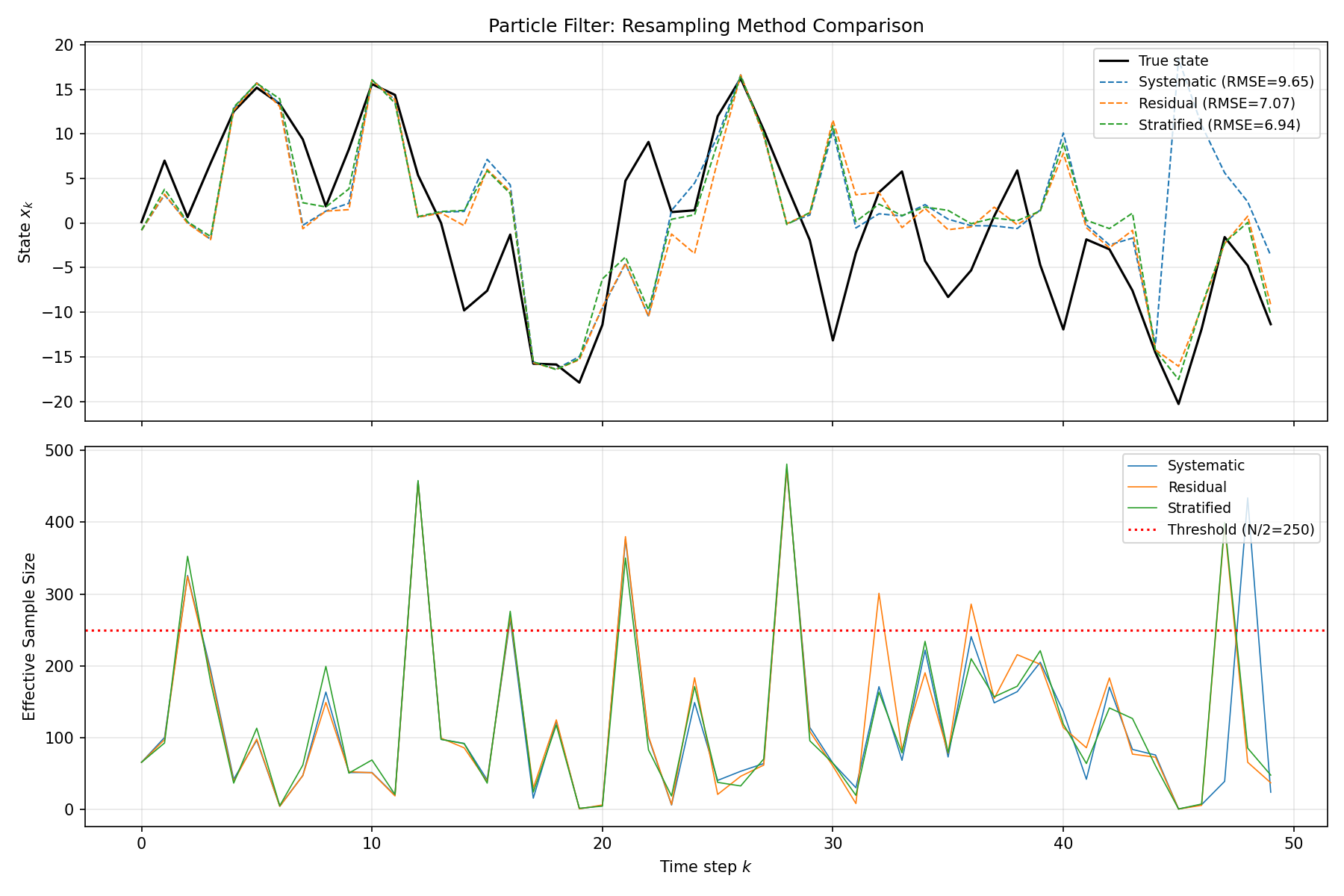
結果の可視化

fig, axes = plt.subplots(2, 1, figsize=(12, 8), sharex=True)

# 状態推定の比較
axes[0].plot(x_true, "k-", linewidth=1.5, label="True state")
colors = {"Systematic": "#2a78d6", "Residual": "#1baf7a",
          "Stratified": "#eda100", "Multinomial": "#e34948"}
for name, res in results.items():
    axes[0].plot(res["estimate"], "--", color=colors[name],
                 linewidth=1, label=f"{name} (RMSE={res['rmse']:.2f})")
axes[0].set_ylabel("State $x_k$")
axes[0].set_title("Particle Filter: Resampling Method Comparison")
axes[0].legend(loc="upper right", fontsize=9)
axes[0].grid(True, alpha=0.3)

# ESSの推移
for name, res in results.items():
    axes[1].plot(res["ess"], color=colors[name], linewidth=0.8, label=name)
axes[1].axhline(y=N_particles / 2, color="red", linestyle=":",
                label=f"Threshold (N/2={N_particles // 2})")
axes[1].set_xlabel("Time step $k$")
axes[1].set_ylabel("Effective Sample Size")
axes[1].legend(loc="upper right", fontsize=9)
axes[1].grid(True, alpha=0.3)

plt.tight_layout()
plt.savefig("particle_filter_comparison.png", dpi=150)
plt.show()

実行結果とロバスト性の検証

上記コードを実際に実行すると（np.random.seed(42) 固定、\(T=100\) 、\(N=500\) ）、以下のRMSEが得られました：

• Systematic: RMSE = 7.5868
• Residual: RMSE = 7.6643
• Stratified: RMSE = 7.2864
• Multinomial: RMSE = 7.4957

この1回の実行だけを見ると、素朴な多項リサンプリングが系統的・残差リサンプリングより良いRMSEを示しており、「多項リサンプリングはオフスプリング分散が大きく劣る」という前節の理論と矛盾するように見えるかもしれません。しかし、これは単一のシード（真の状態系列1本、乱数列1組）に基づく結果であり、統計的な結論を導くには不十分です。そこで、真の状態・観測系列を100通り独立に生成し、各回で4手法すべてを実行してRMSEの分布を比較しました。

n_mc = 100
mc_rmse = {name: np.zeros(n_mc) for name in resamplers}
mc_mean_ess = {name: np.zeros(n_mc) for name in resamplers}
master_seed = np.random.SeedSequence(2026)
child_seeds = master_seed.spawn(n_mc)

for trial in range(n_mc):
    rng = np.random.default_rng(child_seeds[trial])
    xt = np.zeros(T)
    yo = np.zeros(T)
    xt[0] = 0.1
    for k in range(1, T):
        xt[k] = state_transition(xt[k - 1], k) + sigma_w * rng.standard_normal()
    for k in range(T):
        yo[k] = observation(xt[k]) + sigma_v * rng.standard_normal()

    for name, fn in resamplers.items():
        np.random.seed(int(child_seeds[trial].generate_state(1)[0]) ^ hash(name) % (2**31))
        x_est, ess_hist = particle_filter(yo, N_particles, fn)[:2]
        mc_rmse[name][trial] = np.sqrt(np.mean((xt - x_est) ** 2))
        mc_mean_ess[name][trial] = ess_hist.mean()

for name in resamplers:
    r, e = mc_rmse[name], mc_mean_ess[name]
    print(f"{name}: RMSE mean={r.mean():.4f} std={r.std():.4f} mean ESS={e.mean():.2f}")

100回の独立試行の結果は以下の通りです：

4手法間のRMSE平均の差（最大でも約0.18）は、試行間の標準偏差（約1.3〜1.4）に比べて非常に小さいことが分かります。すなわち、この非線形成長モデル・\(N=500\) という条件下では、オフスプリング分散に理論的な差（13.7%〜100%）があるにもかかわらず、フィルタ全体の推定誤差への影響は観測・プロセスノイズによる試行間変動に埋もれてしまうほど小さいということです。これは「リサンプリング手法の選択が本質的に重要でない」ことを意味するのではなく、(1) 本モデルのようにプロセスノイズ \(\sigma_w = \sqrt{10}\) が十分大きく粒子の多様性が毎ステップ再生成される場合は手法間の差が相対的に小さくなること、(2) 差が実際に効いてくるのは、次節で述べる粒子枯渇が深刻化する低ノイズ・高次元・多数回の逐次更新といった条件であることを示唆しています。

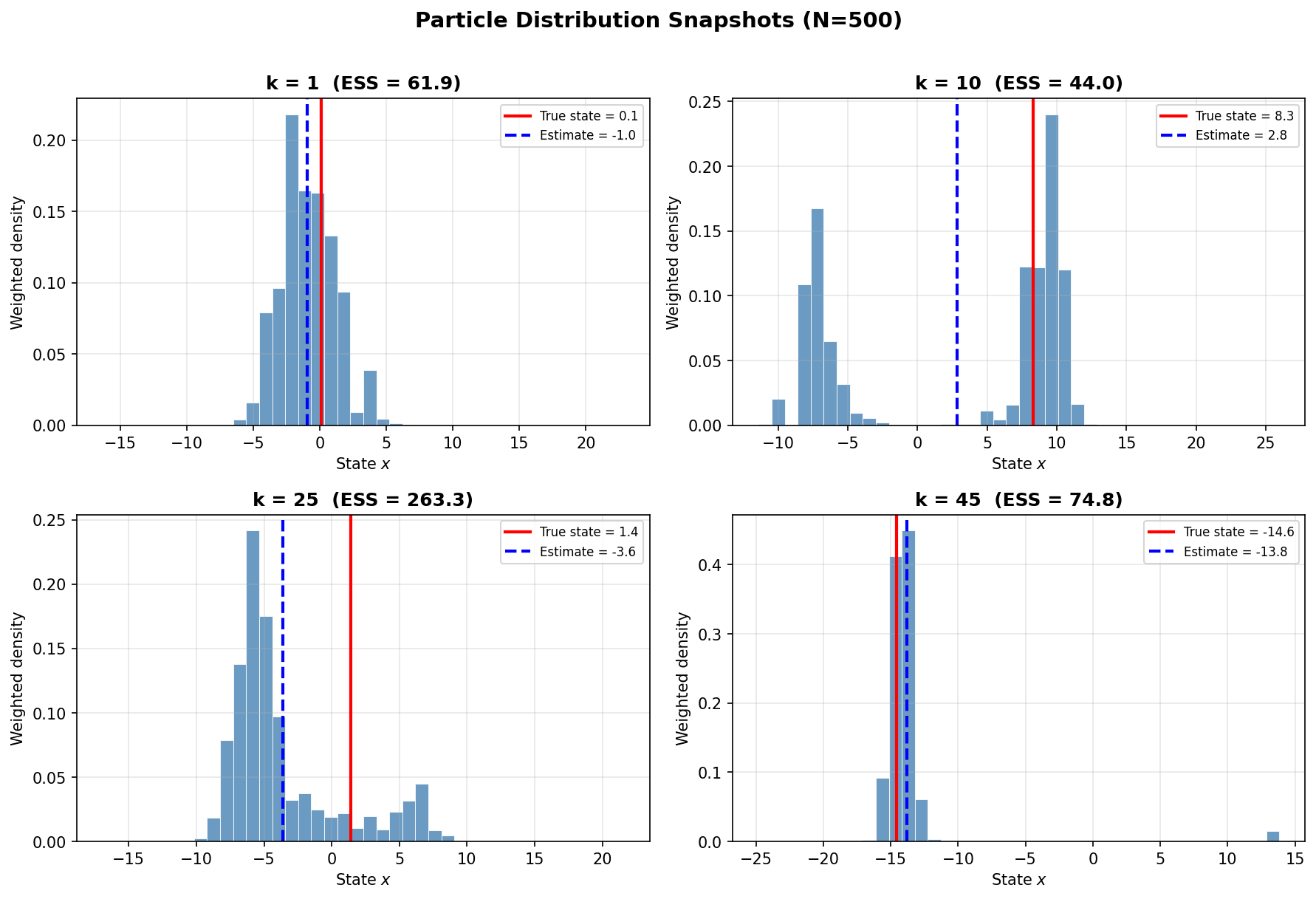
粒子分布のスナップショット

以下の図は、特定の時刻における粒子の分布（重み付きヒストグラム）を示しています。赤線が真の状態、青線が推定値です。

エッジケースと実務上の注意点

粒子枯渇（Sample Impoverishment）

リサンプリングは重みの縮退を解消する一方、新たな問題を生みます。高い重みを持つ粒子を複製し低い重みの粒子を除去するため、リサンプリング直後の粒子集合に含まれる相異なる値の数は、リサンプリング前の \(N_{\text{eff}}\) 以下に制限されます。プロセスノイズが次のステップで十分な多様性を再生成しない限り、この「ユニークな祖先の数の減少」がリサンプリングのたびに複利的に蓄積し、最終的に粒子群が単一の値へ収束（崩壊）します。これを**粒子枯渇（sample impoverishment）あるいは粒子経路の縮退（path degeneracy）**と呼びます。特にプロセスノイズが小さい、あるいは静的パラメータ推定（プロセスノイズが実質ゼロ）のような問題では致命的であり、これが粒子フィルタ単体では静的パラメータ推定に向かない理由です（この課題への対処として、Particle MCMCやSMC²のような手法が提案されています）。

実測として、本記事のシミュレーション（\(T=100\) 、\(N=500\) ）でリサンプリングが発生した回数と、リサンプリング直後に生き残ったユニーク粒子の割合（平均）を測定すると、次のようになりました。

いずれの手法でも、リサンプリング1回につき平均で約78%〜81%の粒子値が失われています。低分散手法（系統的・残差・層化）はいずれも約22%のユニーク粒子を残すのに対し、多項リサンプリングは19.4%とやや低く、前節で導出したオフスプリング分散の理論的な差が、粒子の多様性という観点でも実際に現れることを裏付けています。ただし本モデルではプロセスノイズ \(\sigma_w = \sqrt{10}\) が大きいため、次のステップで多様性がすぐに回復し、深刻な劣化には至っていません（前節のRMSE比較でも手法間の差が小さかった理由の一端はここにあります）。

次元の呪い：理論的な下限

「アルゴリズムの概要」で触れた「高次元への適用が困難」という性質は、直感だけでなく Bengtsson, Bickel & Li (2008) によって定理として証明されています。彼らは、状態次元 \(n\) と粒子数 \(N\) をともに大きくしたとき、（観測尤度がi.i.d.成分を持つなど穏当な仮定のもとで）最大重み \(\max_i \tilde{w}^{(i)}\) が1に収束する、すなわちほぼ全ての確率質量がただ1つの粒子に集中してしまうことを示しました。具体的には、粒子数 \(N\) が次元 \(n\) の指数関数（あるいは特殊な場合でも \(n^{1/3}\) の指数関数）より遅く増加する限り、この収束は避けられません。つまり、次元が2倍になっても粒子数を2倍にすれば済むわけではなく、次元に対して指数的に粒子数を増やす必要があります。

この理論的な予測は、 アンサンブルカルマンフィルタの記事 で40次元Lorenz-96モデルを使って実測されています。粒子数を \(N=20\) から \(N=1000\) へと50倍に増やしても、有効サンプルサイズは平均3.48から20.12へとわずかに改善するのみで、\(N\) に対する割合としてはほぼ変わりません（重み付けを行わないEnKFはこの制約を受けません）。低次元・強非線形の問題には本記事の粒子フィルタが適する一方、高次元問題ではEnKFやUKFのような重みなしの手法を検討すべき理由がここにあります。

リサンプリング閾値の選び方

本記事では \(N_{\text{eff}} < N/2\) を閾値として採用しましたが、これは経験則であり万能ではありません。閾値を低く（例えば \(N/10\) ）設定すると、リサンプリングの頻度が下がり粒子枯渇は緩和されますが、重みの縮退した状態のまま多くのステップを過ごすことになり推定量の分散が増えます。逆に閾値を高く（例えば毎ステップ、つまり常にリサンプリングする）設定すると、縮退は最小限に抑えられる一方、前述の粒子枯渇が加速します。この閾値の選択と、オフスプリング分散の低い手法（系統的・残差）の選択は独立した設計上の判断であり、両方を適切に選んで初めて粒子フィルタは安定して動作します。

提案分布と事前分布のミスマッチ

本記事の実装では初期粒子を \(\mathcal{N}(0, 5)\) （標準偏差 \(\approx 2.24\) ）からサンプリングしていますが、真の状態は \(\pm 20\) 程度まで変動します。事前分布が真の状態の存在範囲を十分にカバーしていない場合、初期ステップで全粒子の尤度が同時に低くなり、\(k=0\) の時点で深刻な縮退が生じることがあります。実務では、事前分布の広さと観測ノイズの大きさのバランスを事前に確認しておくことが重要です。

微分可能なリサンプリング：勾配ベース学習への拡張

本記事の系統的・層化・多項リサンプリングは、いずれも「累積分布関数のどの区間に位置するか」という閾値判定（if positions[i] < cumsum[j]）や np.random.choice によるカテゴリカルサンプリングを含み、この操作は入力の重み weights に関して微分不可能です。これは、ニューラルネットワークで状態遷移関数 \(f\) や観測関数 \(h\) 、あるいは提案分布そのものを学習しようとするとき、勾配がリサンプリングのステップで遮断されてしまうことを意味します。この問題への対処は2020年代に入って活発な研究領域になっており、直近では Csuzdi, Törő & Bécsi (2024) が、経験分布関数（empirical CDF）からの決定論的なサンプリング配置を微分可能な形に再構成する “Optimal Placement Resampling” を提案し、勾配ベースのパラメータ推定・提案分布学習に応用しています。本記事の系統的リサンプリングと発想が近い（CDF上に決定論的な位置を配置する）手法を、自動微分と両立する形に再設計している点が興味深く、古典的なリサンプリング手法が深層学習との統合に向けて今も拡張され続けていることを示しています。

フィルタ手法の比較

粒子フィルタと、ガウス近似に基づくフィルタ手法との比較を以下にまとめます。

粒子フィルタは分布の仮定を必要としない汎用性が強みですが、高次元問題では粒子数が指数的に増加する「次元の呪い」に直面します。低次元で強い非線形性や非ガウス性がある問題では粒子フィルタが有効で、高次元の穏やかな非線形問題ではCKFやUKFが適しています。

関連記事

• カルマンフィルタの理論とPython実装 - 線形ガウスの場合の最適フィルタであるカルマンフィルタを解説しています。
• 拡張カルマンフィルタ（EKF）の理論とPython実装 - 非線形システムへの線形化ベースのアプローチを解説しています。
• Unscented Kalman Filter（UKF）の理論とPython実装 - シグマポイントベースの非線形フィルタを解説しています。
• カルマンスムーザ（RTS Smoother）の理論とPython実装 - 全時刻の観測データを使った平滑化手法を解説しています。
• カルマンスムーザの比較 - 粒子スムーザにつながるスムージング手法群を横断比較しています。
• 非線形カルマンスムーザ（Extended RTS Smoother・Unscented RTS Smoother） - EKF/UKFをスムージングに拡張した手法。非ガウス性が強い場合の粒子スムーザとの使い分けの指針になります。
• MCMC入門：メトロポリス・ヘイスティングス法とギブスサンプリング - 粒子フィルタと同じくモンテカルロサンプリングを基盤とする手法です。
• ガウス過程回帰の理論とPython実装 - ガウス分布の仮定下で柔軟な非線形回帰を扱う手法。粒子フィルタが分布の仮定を捨てるのに対し、GPは閉形式で予測分散を得られます。
• ベイズ最適化の基礎とPython実装 - サンプル効率を重視する逐次推定の対比対象。粒子フィルタが状態推定、ベイズ最適化が関数最適化と棲み分けます。
• 時系列データの異常検知：統計的手法からカルマンフィルタまで - 粒子フィルタの尤度評価を異常検知のスコアとして使う応用例につながります。
• モンテカルロ最適化メソッド比較（CEM/SA/GA/MPPI/PSO） - 粒子フィルタと同じ重点サンプリング枠組みを最適化側に展開した5手法のハブ記事。状態推定と関数最適化での Monte Carlo の使われ方を対比できます。
• 機械学習による時系列予測・分類・異常検知ハブ - 粒子フィルタを線形カルマン・EKF・UKF・LSTM・Isolation Forest と並べ、非ガウス・強非線形の状態空間における異常検知・予測の選び方を整理したハブ記事。
• アンサンブルカルマンフィルタ（EnKF）の理論とPython実装 - 本記事の次元の呪いを、重み付けを行わないアンサンブル共分散近似で回避する手法。40次元Lorenz-96モデルで両者の挙動を直接比較しています。

参考文献

• Arulampalam, M. S., Maskell, S., Gordon, N., & Clapp, T. (2002). “A Tutorial on Particle Filters for Online Nonlinear/Non-Gaussian Bayesian Tracking.” IEEE Transactions on Signal Processing, 50(2), 174-188.
• Doucet, A., & Johansen, A. M. (2009). “A Tutorial on Particle Filtering and Smoothing: Fifteen Years Later.” Handbook of Nonlinear Filtering, 12(656-704), 3.
• Douc, R., & Cappe, O. (2005). “Comparison of Resampling Schemes for Particle Filtering.” Proceedings of the 4th International Symposium on Image and Signal Processing and Analysis, 64-69.
• Gordon, N. J., Salmond, D. J., & Smith, A. F. M. (1993). “Novel Approach to Nonlinear/Non-Gaussian Bayesian State Estimation.” IEE Proceedings F (Radar and Signal Processing), 140(2), 107-113.
• Kong, A., Liu, J. S., & Wong, W. H. (1994). “Sequential Imputations and Bayesian Missing Data Problems.” Journal of the American Statistical Association, 89(425), 278-288.
• Doucet, A., Godsill, S., & Andrieu, C. (2000). “On Sequential Monte Carlo Sampling Methods for Bayesian Filtering.” Statistics and Computing, 10(3), 197-208.
• Bengtsson, T., Bickel, P., & Li, B. (2008). “Curse-of-Dimensionality Revisited: Collapse of the Particle Filter in Very Large Scale Systems.” IMS Collections: Probability and Statistics: Essays in Honor of David A. Freedman, 2, 316-334.
• Csuzdi, D., Törő, O., & Bécsi, T. (2024). “Differentiable Particle Filtering Using Optimal Placement Resampling.” arXiv preprint arXiv:2402.16639.