はじめに
粒子群最適化(Particle Swarm Optimization, PSO)は、鳥や魚の群れの集合行動から着想を得たメタヒューリスティクス最適化手法です。Kennedy と Eberhart によって 1995 年に提案され、勾配情報を必要としないブラックボックス最適化アルゴリズムとして、連続値の多峰性問題で広く用いられてきました。
PSO の特徴は、各**粒子(particle)**が「位置」と「速度」を持ち、自分自身が見つけたこれまでの最良解(個人最良 pbest)と、群れ全体が共有する最良解(全体最良 gbest)の双方に引き寄せられながら探索空間を移動する点にあります。これにより、ランダム探索だけでは到達しにくい大域解の周辺へ、群れ全体の知能で素早く収束していきます。
本稿では PSO の更新式を慣性重み \(w\) 、認知係数 \(c_1\) 、社会係数 \(c_2\) の役割から丁寧に整理し、Sphere 関数と Rastrigin 関数の最小化を題材に Python 実装と収束の様子を可視化します。
アルゴリズム
粒子の状態
集団サイズを \(N\) 、探索空間の次元を \(D\) とします。各粒子 \(i \in \{1, \dots, N\}\) は、
- 位置 \(\mathbf{x}_i^t \in \mathbb{R}^D\)
- 速度 \(\mathbf{v}_i^t \in \mathbb{R}^D\)
- 個人最良位置 \(\mathbf{p}_i^t\) (粒子 \(i\) がこれまでに到達した最良位置)
を保持します。さらに群れ全体で共有する全体最良位置 \(\mathbf{g}^t = \arg\min_{i} f(\mathbf{p}_i^t)\) を持ちます。
速度更新
速度は次の式で更新されます。
$$ \mathbf{v}_i^{t+1} = w , \mathbf{v}_i^{t}
- c_1 \mathbf{r}_1 \odot (\mathbf{p}_i^{t} - \mathbf{x}_i^{t})
- c_2 \mathbf{r}_2 \odot (\mathbf{g}^{t} - \mathbf{x}_i^{t}) \tag{1} $$
ここで \(\mathbf{r}_1, \mathbf{r}_2 \sim U[0,1]^D\) は次元ごとに独立な一様乱数ベクトル、\(\odot\) は要素積です。右辺の各項は次の意味を持ちます。
- 第1項 \(w \, \mathbf{v}_i^t\) : 慣性項。直前の速度をどれだけ引き継ぐか
- 第2項 \(c_1 \mathbf{r}_1 \odot (\mathbf{p}_i^t - \mathbf{x}_i^t)\) : 認知項。自分自身の経験(pbest)への引力
- 第3項 \(c_2 \mathbf{r}_2 \odot (\mathbf{g}^t - \mathbf{x}_i^t)\) : 社会項。群れ全体の経験(gbest)への引力
位置更新
位置は速度を用いて単純に進めます。
\[ \mathbf{x}_i^{t+1} = \mathbf{x}_i^{t} + \mathbf{v}_i^{t+1} \tag{2} \]pbest と gbest の更新
各イテレーションで、粒子の現在位置の評価値が個人最良を更新したら \(\mathbf{p}_i\) を置き換えます。
\[ \mathbf{p}_i^{t+1} = \begin{cases} \mathbf{x}_i^{t+1} & \text{if } f(\mathbf{x}_i^{t+1}) < f(\mathbf{p}_i^{t}) \\ \mathbf{p}_i^{t} & \text{otherwise} \end{cases} \tag{3} \]そして全体最良も同様に更新します。
\[ \mathbf{g}^{t+1} = \arg\min_{i} f(\mathbf{p}_i^{t+1}) \tag{4} \]ハイパーパラメータの役割
慣性重み \(w\)
\(w\) は探索の 多様性(exploration) と 集中(exploitation) のバランスを制御します。
- \(w\) が大きい(例: \(w \approx 0.9\) ): 粒子が直前の速度を強く保つため、広域探索が促進される
- \(w\) が小さい(例: \(w \approx 0.4\) ): 速度が急速に減衰し、局所的な精緻化が進む
実用上は、序盤に広く探索し終盤に収束させるため、線形に減衰させる線形減衰慣性重み(linearly decreasing inertia weight, LDIW) が定石です。
\[ w_t = w_{\max} - (w_{\max} - w_{\min}) \cdot \frac{t}{T_{\max}} \tag{5} \]典型値は \(w_{\max} = 0.9, w_{\min} = 0.4\) です。
認知係数 \(c_1\) と社会係数 \(c_2\)
\(c_1\) と \(c_2\) は、それぞれ自分自身の経験と群れの経験への引力の強さを決めます。
- \(c_1 \gg c_2\) : 各粒子が自分の経験を重視し、独立的な探索が進む
- \(c_1 \ll c_2\) : 群れの最良解への収束が支配的となり、局所解に集中しやすい
Clerc & Kennedy (2002) は、収束性の解析から \(c_1 = c_2 = 2.05\) 、慣性重み \(w = 0.7298\) という**収束係数(constriction coefficient)**を提案しています。実装時のデフォルトとしては \(w = 0.729, c_1 = c_2 = 1.4944\) がよく使われます。
速度のクリッピング
粒子が探索領域外へ発散することを防ぐため、各次元の速度を \(|v_{i,d}| \leq v_{\max}\) にクリップする運用が一般的です。\(v_{\max}\) は探索範囲幅の 10〜20% 程度が目安です。
ベンチマーク関数
Sphere 関数(単峰性)
\[ f_{\text{sphere}}(\mathbf{x}) = \sum_{i=1}^{D} x_i^2 \tag{6} \]大域最小値は \(f(\mathbf{0}) = 0\) 。単峰性なので PSO は容易に収束します。
Rastrigin 関数(多峰性)
\[ f_{\text{rastrigin}}(\mathbf{x}) = 10 D + \sum_{i=1}^{D} \left[ x_i^2 - 10 \cos(2\pi x_i) \right] \tag{7} \]大域最小値は \(f(\mathbf{0}) = 0\) ですが、無数の局所解を持つため、慣性重みや係数の設定によっては粒子が早期に局所解に集中して停滞することがあります。
Python 実装
NumPy のみを用いた基本的な PSO 実装です。線形減衰慣性重みと速度クリッピングを組み込んでいます。
import numpy as np
import matplotlib.pyplot as plt


def sphere(x):
    """Sphere 関数(単峰性)"""
    return np.sum(x**2, axis=-1)


def rastrigin(x):
    """Rastrigin 関数(多峰性)"""
    return 10 * x.shape[-1] + np.sum(x**2 - 10 * np.cos(2 * np.pi * x), axis=-1)


class PSO:
    def __init__(self, dim, n_particles=40, bounds=(-5.12, 5.12),
                 w_max=0.9, w_min=0.4, c1=1.4944, c2=1.4944,
                 v_max_ratio=0.2):
        self.dim = dim
        self.n_particles = n_particles
        self.bounds = bounds
        self.w_max = w_max
        self.w_min = w_min
        self.c1 = c1
        self.c2 = c2
        # 速度上限は探索範囲幅の v_max_ratio 倍
        self.v_max = v_max_ratio * (bounds[1] - bounds[0])

    def initialize(self):
        low, high = self.bounds
        x = np.random.uniform(low, high, (self.n_particles, self.dim))
        v = np.random.uniform(-self.v_max, self.v_max,
                              (self.n_particles, self.dim))
        return x, v

    def run(self, objective, max_iter=200):
        x, v = self.initialize()
        f = objective(x)

        # pbest / gbest 初期化
        pbest = x.copy()
        pbest_f = f.copy()
        g_idx = int(np.argmin(pbest_f))
        gbest = pbest[g_idx].copy()
        gbest_f = float(pbest_f[g_idx])

        history = [gbest_f]

        for t in range(max_iter):
            # 線形減衰慣性重み
            w = self.w_max - (self.w_max - self.w_min) * (t / max_iter)

            # 速度更新(式 1)
            r1 = np.random.random((self.n_particles, self.dim))
            r2 = np.random.random((self.n_particles, self.dim))
            v = (w * v
                 + self.c1 * r1 * (pbest - x)
                 + self.c2 * r2 * (gbest - x))
            v = np.clip(v, -self.v_max, self.v_max)

            # 位置更新(式 2)
            x = x + v
            x = np.clip(x, *self.bounds)

            # 評価と pbest / gbest 更新
            f = objective(x)
            improved = f < pbest_f
            pbest[improved] = x[improved]
            pbest_f[improved] = f[improved]

            g_idx = int(np.argmin(pbest_f))
            if pbest_f[g_idx] < gbest_f:
                gbest = pbest[g_idx].copy()
                gbest_f = float(pbest_f[g_idx])

            history.append(gbest_f)

        return gbest, gbest_f, history


# --- 実行 ---
np.random.seed(42)
pso_sphere = PSO(dim=10)
_, best_sphere, hist_sphere = pso_sphere.run(sphere, max_iter=200)

np.random.seed(42)
pso_rastrigin = PSO(dim=10)
_, best_rastrigin, hist_rastrigin = pso_rastrigin.run(rastrigin, max_iter=200)

print(f"Sphere    最良適応度: {best_sphere:.6e}")
print(f"Rastrigin 最良適応度: {best_rastrigin:.6e}")

# --- 収束曲線のプロット ---
plt.figure(figsize=(10, 5))
plt.plot(hist_sphere, label='Sphere (10D)')
plt.plot(hist_rastrigin, label='Rastrigin (10D)')
plt.xlabel('Iteration')
plt.ylabel('Best Objective Value')
plt.title('PSO Convergence on Sphere and Rastrigin')
plt.yscale('log')
plt.grid(True, alpha=0.3)
plt.legend()
plt.tight_layout()
plt.show()
実際に上記コードを実行すると(seed=42、10次元、粒子数40、200イテレーション)、次の結果が得られます。
Sphere    最良適応度: 2.547928e-15
Rastrigin 最良適応度: 6.964713e+00
Sphere 関数は単峰性のため \(10^{-15}\) 程度まで収束する一方、Rastrigin 関数は多峰性により大域最小値 \(0\) には遠く及ばず、\(7\) 程度の局所解近傍で停滞しています。慣性重みの初期値・粒子数・係数の調整が結果を大きく左右する点は、次節以降で定量的に検証します。
慣性重みが収束に与える影響
固定の \(w\) を変化させた場合の比較も簡単に再現できます。
import numpy as np
import matplotlib.pyplot as plt

results = {}
for w in [0.3, 0.5, 0.7, 0.9]:
    np.random.seed(0)
    pso = PSO(dim=10, w_max=w, w_min=w)  # 固定慣性重み
    _, _, history = pso.run(rastrigin, max_iter=200)
    results[w] = history

plt.figure(figsize=(10, 5))
for w, history in results.items():
    plt.plot(history, label=f'w = {w}')
plt.xlabel('Iteration')
plt.ylabel('Best Objective Value')
plt.title('Effect of Inertia Weight on Rastrigin (10D)')
plt.yscale('log')
plt.grid(True, alpha=0.3)
plt.legend()
plt.tight_layout()
plt.show()
同じ seed=0 で実行した結果、200イテレーション後の最良適応度は次のようになりました。
| \(w\) (固定) | 最終最良適応度 |
|---|---|
| 0.3 | 3.981448 |
| 0.5 | 15.919330 |
| 0.7 | 4.974795 |
| 0.9 | 35.174607 |
\(w = 0.9\) では速度が減衰しにくく局所探索が進まないため最も悪化し、\(w = 0.5\) も中途半端に探索と収束のバランスを崩して悪い結果になりました。\(w = 0.3\) と \(w = 0.7\) が相対的に良好ですが、これは単一シードの結果であり、\(w\) と最終適応度の関係は単調ではありません(次節で見るように、固定 \(w\) は「早期に多様性を失って停滞するリスク」と「収束が遅すぎるリスク」の間でシード依存性が大きく、LDIW のように時間的に調整する方が頑健です)。
収束・発散の安定性解析
前節では固定 \(w\) を実験的に振りましたが、そもそも速度更新式(式1, 式2)はどのようなパラメータ領域で収束し、どこから発散するのでしょうか。ここでは van den Bergh (2001)、Clerc & Kennedy (2002)、Trelea (2003) らの標準的な安定性解析に沿って境界を導出し、数値実験で確認します。
単純化モデルによる導出
厳密な解析のため、次の標準的な単純化を行います。
- 1次元・1粒子に着目する(各次元・各粒子は式の上で独立に振る舞うため一般性を失いません)
- 個人最良 \(\mathbf{p}_i\) と全体最良 \(\mathbf{g}\) が同一の点 \(p\) に固定されている(探索が局所的に停滞した局面を想定した安定性解析)
- 乱数 \(r_1, r_2 \sim U[0,1]\) をその期待値 \(E[r_1] = E[r_2] = 0.5\) で置き換える(決定論的近似)
偏差 \(e_t = x_t - p\) を定義すると、式(1)の第2・3項は \(c_1 r_1 (p - x_t) + c_2 r_2 (p - x_t) \to -\phi\, e_t\) (ただし \(\phi = (c_1+c_2)/2\) )とまとまるので、更新式は
\[ v_{t+1} = w\, v_t - \phi\, e_t \] \[ e_{t+1} = e_t + v_{t+1} = w\, v_t + (1-\phi)\, e_t \]行列形式では
$$ \begin{pmatrix} v_{t+1} \ e_{t+1} \end{pmatrix}
\begin{pmatrix} w & -\phi \ w & 1-\phi \end{pmatrix} \begin{pmatrix} v_t \ e_t \end{pmatrix} \tag{8} $$
となります。
固有値と安定性条件
この線形漸化式が \(t \to \infty\) で \(e_t \to 0\) に収束する必要十分条件は、係数行列の固有値 \(\lambda\) がすべて単位円内(\(|\lambda| < 1\) )にあることです。トレース \(w+1-\phi\) 、行列式 \(w\) より、特性方程式は
\[ \lambda^2 - (1 + w - \phi)\lambda + w = 0 \tag{9} \]となります。2次方程式 \(\lambda^2 - b_1 \lambda + b_0 = 0\) の根が単位円内に収まるための Jury の安定性判別条件は \(|b_0| < 1\) 、\(1 - b_1 + b_0 > 0\) 、\(1 + b_1 + b_0 > 0\) の3本です。式(9)の \(b_1 = 1+w-\phi\) 、\(b_0 = w\) を代入すると、
- \(|w| < 1\)
- \(1-(1+w-\phi)+w = \phi > 0\)
- \(1+(1+w-\phi)+w = 2+2w-\phi > 0 \iff \phi < 2(1+w)\)
の3条件が得られます。\(\phi = (c_1+c_2)/2\) を戻すと、次の安定性条件が導かれます。
\[ w < 1, \qquad 0 < c_1 + c_2 < 4(1+w) \]この結果は Engelbrecht (2007) の教科書 Computational Intelligence: An Introduction 第16章でも、van den Bergh の収束解析を要約する形で同じ不等式(式16.38–16.39)として紹介されています。Clerc & Kennedy (2002) の収束係数 \(w=0.7298, c_1=c_2=2.05\) (\(c_1+c_2=4.10\) 、境界 \(4(1+w)=6.92\) )や、本記事のデフォルト \(w=0.729, c_1=c_2=1.4944\) (\(c_1+c_2 \approx 2.99\) )は、いずれもこの安定領域の内側に十分な余裕を持って収まっています。
数値実験:境界付近・境界外での発散
上記の単純化モデル(式8)をそのまま実装し、\(e_0=1\) から出発した偏差 \(|e_t|\) の推移を確認します。
import numpy as np


def simulate_deviation(w, c1, c2, T=150, seed=0, e0=1.0):
    """簡略化モデル(式8)の偏差 e_t = x_t - p を追跡する。
    pbest = gbest = p で固定した局所安定性解析の設定に対応する。"""
    rng = np.random.default_rng(seed)
    v, e = 0.0, e0
    traj = [abs(e)]
    for _ in range(T):
        r1, r2 = rng.random(), rng.random()
        v = w * v - (c1 * r1 + c2 * r2) * e
        e = e + v
        traj.append(abs(e) + 1e-300)
    return np.array(traj)


configs = [
    ("Clerc-Kennedy (w=0.7298, c1=c2=1.4962)", 0.7298, 1.4962, 1.4962),
    ("w=0.70, c1=c2=3.0 (境界内)", 0.70, 3.0, 3.0),
    ("w=0.70, c1=c2=4.0 (境界超過)", 0.70, 4.0, 4.0),
]

for label, w, c1, c2 in configs:
    bound = 4 * (1 + w)
    finals = [simulate_deviation(w, c1, c2, T=150, seed=s)[-1] for s in range(50)]
    print(f"{label:42} c1+c2={c1+c2:.2f} bound={bound:.2f} "
          f"median|e_150|={np.median(finals):.3e}")
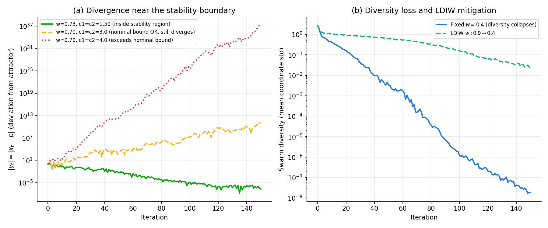
実行結果(50シードの中央値)は次の通りです。
Clerc-Kennedy (w=0.7298, c1=c2=1.4962)    c1+c2=2.99 bound=6.92 median|e_150|=2.374e-07
w=0.70, c1=c2=3.0 (境界内)                 c1+c2=6.00 bound=6.80 median|e_150|=1.047e+12
w=0.70, c1=c2=4.0 (境界超過)                c1+c2=8.00 bound=6.80 median|e_150|=2.010e+35
Clerc-Kennedy の係数は \(10^{-7}\) 程度まで滑らかに収束する一方、\(c_1=c_2=3.0\) (\(w=0.7\) )は式(9)の境界 \(4(1+w)=6.8\) を満たしているにもかかわらず、実際には \(50\) シード中央値で \(10^{12}\) まで発散しました。\(c_1=c_2=4.0\) は \(10^{35}\) とさらに激しく発散します。
これは式(9)の解析が乱数 \(r_1, r_2\) を期待値 \(0.5\) で置き換えた決定論的(期待値)近似にすぎないためです。実際の PSO は毎ステップ乱数を引き直す確率的漸化式であり、Jiang, Luo & Yang (2007) や Poli (2009) が指摘するように、期待値の軌道が収束していても、軌道の分散は発散しうることが知られています(Cleghorn & Engelbrecht はこれを「1次安定性(order-1 stability)」と「2次安定性(order-2 stability)」の違いとして整理しています)。式 \(0 < c_1+c_2 < 4(1+w)\) は必要条件の目安ではあっても、確率的な発散を防ぐには不十分な場合があるということです。実務上は、Clerc-Kennedy や本記事のデフォルトのように、境界よりも十分小さい \(c_1+c_2\) を選ぶか、速度クリッピングを併用するのが安全です。
下図(a)は、この3設定について \(|e_t|\) の推移を1シードで可視化したものです。
多様性喪失と早期収束
安定性解析とは別に、PSO には全粒子が同じ局所解(gbest の周辺)に集まってしまい、探索が止まるという早期収束(premature convergence)のリスクがあります。式(1)の社会項 \(c_2 r_2 (\mathbf{g}^t - \mathbf{x}_i^t)\) が全粒子を同じ点に引き寄せる一方、慣性項 \(w \mathbf{v}_i^t\) が小さいと速度がすぐに減衰するため、粒子間の距離(多様性)が急速に失われます。多様性が失われた後は、認知項・社会項の駆動力そのものがほぼゼロになり、群れは新しい領域を探索できなくなります。
数値実験:多様性の崩壊とLDIWによる緩和
粒子数を少なく(\(N=10\) )し、10次元 Rastrigin 関数上で、慣性重みを (a) \(w=0.4\) に固定した場合と (b) 線形減衰慣性重み(LDIW, \(w: 0.9 \to 0.4\) )を用いた場合を比較します。多様性の指標として、各次元の座標の標準偏差を次元平均した値 \(\bar{\sigma}_t = \frac{1}{D}\sum_{d=1}^{D} \mathrm{std}(x_{1,d}^t, \dots, x_{N,d}^t)\) を追跡します。
import numpy as np


def rastrigin(x):
    return 10 * x.shape[-1] + np.sum(x**2 - 10 * np.cos(2 * np.pi * x), axis=-1)


def run_pso_track_diversity(dim, n_particles, w_max, w_min, decay, c1, c2,
                             max_iter=150, bounds=(-5.12, 5.12), v_max_ratio=0.2, seed=0):
    rng = np.random.default_rng(seed)
    low, high = bounds
    v_max = v_max_ratio * (high - low)
    x = rng.uniform(low, high, (n_particles, dim))
    v = rng.uniform(-v_max, v_max, (n_particles, dim))
    f = rastrigin(x)
    pbest, pbest_f = x.copy(), f.copy()
    g_idx = int(np.argmin(pbest_f))
    gbest_f = float(pbest_f[g_idx])
    diversity = [float(np.mean(np.std(x, axis=0)))]
    for t in range(max_iter):
        w = w_max - (w_max - w_min) * (t / max_iter) if decay else w_max
        r1 = rng.random((n_particles, dim))
        r2 = rng.random((n_particles, dim))
        v = w * v + c1 * r1 * (pbest - x) + c2 * r2 * (pbest[g_idx] - x)
        v = np.clip(v, -v_max, v_max)
        x = np.clip(x + v, low, high)
        f = rastrigin(x)
        improved = f < pbest_f
        pbest[improved], pbest_f[improved] = x[improved], f[improved]
        g_idx = int(np.argmin(pbest_f))
        gbest_f = min(gbest_f, float(pbest_f[g_idx]))
        diversity.append(float(np.mean(np.std(x, axis=0))))
    return gbest_f, diversity


N_SEEDS = 30
for label, w_max, decay in [("fixed w=0.4", 0.4, False), ("LDIW w:0.9->0.4", 0.9, True)]:
    finals, collapse_iters = [], []
    for seed in range(N_SEEDS):
        best_f, diversity = run_pso_track_diversity(
            dim=10, n_particles=10, w_max=w_max, w_min=0.4, decay=decay,
            c1=1.4944, c2=1.4944, max_iter=150, seed=seed)
        finals.append(best_f)
        threshold = 0.01 * diversity[0]
        collapse_iters.append(next((i for i, d in enumerate(diversity) if d < threshold), len(diversity)))
    print(f"{label:16} collapse_iter(mean)={np.mean(collapse_iters):.1f}  "
          f"final_f(mean±std)={np.mean(finals):.2f}±{np.std(finals):.2f}")
実行結果は次の通りです。
fixed w=0.4      collapse_iter(mean)=30.6  final_f(mean±std)=20.77±10.64
LDIW w:0.9->0.4  collapse_iter(mean)=120.1  final_f(mean±std)=16.66±6.81
30シードで平均した結果は次の通りです(\(N=10\)
, \(c_1=c_2=1.4944\)
, max_iter=150, Rastrigin 10D)。
| 設定 | 多様性が初期値の1%未満になるまでの平均イテレーション数 | 最終最良適応度(平均±標準偏差) |
|---|---|---|
| 固定 \(w=0.4\) (減衰なし) | 30.6 | \(20.77 \pm 10.64\) |
| LDIW(\(w: 0.9\to 0.4\) ) | 120.1 | \(16.66 \pm 6.81\) |
固定 \(w=0.4\) では平均30イテレーション程度で多様性が初期値の1%未満まで崩壊し、その後は粒子群がほぼ1点に凝集したまま局所解付近で停滞します。LDIW ではこの崩壊が平均120イテレーションまで遅延され、探索期間が実質的に4倍近く確保される結果、最終適応度も平均・分散ともに改善しています(ただし LDIW でも最終的には多様性を失うこと自体は避けられず、あくまで崩壊までの猶予を延ばす緩和策である点に注意が必要です)。
図(b)(前節の図と共通)に、多様性 \(\bar{\sigma}_t\) の推移(両設定の30シード平均)を示しました。固定 \(w=0.4\) は指数関数的に急落する一方、LDIW は序盤の高い \(w\) により多様性を長く保持し、終盤にかけて緩やかに収束していく様子が対比できます。
多様性喪失への対策としては、本記事で扱った LDIW のほかにも、粒子の速度をランダムに再初期化する手法や、探索担当・収束担当で役割を分けた**協調型二群 PSO(TCPSO)**などが知られています。TCPSO の詳細な仕組み・収束条件の導出・局所解への実践的対策は、 協調型二群粒子群最適化(TCPSO)の数理:スレーブ/マスター群の収束条件の導出とPython実装 で扱っています。
他の最適化手法との比較
| 手法 | 集団ベース | 主なメカニズム | 多峰性への耐性 | 評価コストが高い問題 |
|---|---|---|---|---|
| PSO | Yes | 速度・位置の更新(pbest/gbest) | 中 | 不向き |
| GA | Yes | 選択・交叉・突然変異 | 高 | 不向き |
| CEM | Yes | 確率分布の反復更新 | 中 | 不向き |
| SA | No | 温度付き確率的受容 | 高 | 不向き |
| ベイズ最適化 | No | ガウス過程による代理モデル | 中 | 得意 |
PSO は実装が極めて簡潔でハイパーパラメータも少なく、連続値の中規模次元問題に対して高い実用性を持ちます。一方で、評価が極端に高コストな問題(実機実験など)では、評価回数を抑えられるベイズ最適化の方が有利です。
実行検証:GA・SAとの評価回数を揃えた比較
遺伝的アルゴリズム(GA)の基礎とPython実装
と
焼きなまし法(Simulated Annealing)の仕組みとPython実装
では、それぞれ独立に Rastrigin 関数(10次元)でのベンチマークが行われていますが、GA は pop_size=200, max_generations=300(評価回数 \(60{,}000\)
回)、SA は max_iter=10000(評価回数 \(10{,}000\)
回)と条件が異なり、単純比較はできません。そこで3手法とも評価回数を約8000回に統一(PSO: 粒子数40×200イテレーション、GA: 個体数40×世代数200、SA: 反復回数8000)した上で、Sphere 関数と Rastrigin 関数(いずれも10次元)を10シードずつ実行し比較しました。
import numpy as np


def sphere(x):
    return np.sum(x**2, axis=-1)


def rastrigin(x):
    return 10 * x.shape[-1] + np.sum(x**2 - 10 * np.cos(2 * np.pi * x), axis=-1)


def run_pso(objective, dim, n_particles=40, max_iter=200, bounds=(-5.12, 5.12),
            w_max=0.9, w_min=0.4, c1=1.4944, c2=1.4944, v_max_ratio=0.2, seed=0):
    rng = np.random.default_rng(seed)
    low, high = bounds
    v_max = v_max_ratio * (high - low)
    x = rng.uniform(low, high, (n_particles, dim))
    v = rng.uniform(-v_max, v_max, (n_particles, dim))
    f = objective(x)
    pbest, pbest_f = x.copy(), f.copy()
    g_idx = int(np.argmin(pbest_f))
    gbest_f = float(pbest_f[g_idx])
    for t in range(max_iter):
        w = w_max - (w_max - w_min) * (t / max_iter)
        r1 = rng.random((n_particles, dim))
        r2 = rng.random((n_particles, dim))
        v = w * v + c1 * r1 * (pbest - x) + c2 * r2 * (pbest[g_idx] - x)
        v = np.clip(v, -v_max, v_max)
        x = np.clip(x + v, low, high)
        f = objective(x)
        improved = f < pbest_f
        pbest[improved], pbest_f[improved] = x[improved], f[improved]
        g_idx = int(np.argmin(pbest_f))
        gbest_f = min(gbest_f, float(pbest_f[g_idx]))
    return gbest_f


def run_ga(objective, dim, pop_size=40, max_generations=200, bounds=(-5.12, 5.12), seed=0):
    rng = np.random.default_rng(seed)
    low, high = bounds

    def tournament(population, fitness, k=3):
        idx = rng.integers(0, pop_size, k)
        return population[idx[np.argmin(fitness[idx])]]

    def crossover(p1, p2, alpha=0.5):
        lo = np.minimum(p1, p2) - alpha * np.abs(p1 - p2)
        hi = np.maximum(p1, p2) + alpha * np.abs(p1 - p2)
        return np.clip(rng.uniform(lo, hi), low, high)

    def mutate(ind, sigma=0.1, rate=0.1):
        mask = rng.random(dim) < rate
        ind = ind.copy()
        ind[mask] += rng.normal(0, sigma * (high - low), size=mask.sum())
        return np.clip(ind, low, high)

    population = rng.uniform(low, high, (pop_size, dim))
    best_f = float(np.min(objective(population)))
    for _ in range(max_generations):
        fitness = objective(population)
        best_idx = int(np.argmin(fitness))
        best_f = min(best_f, float(fitness[best_idx]))
        new_pop = [population[best_idx].copy()]  # エリート保存
        while len(new_pop) < pop_size:
            child = mutate(crossover(tournament(population, fitness), tournament(population, fitness)))
            new_pop.append(child)
        population = np.array(new_pop[:pop_size])
    return min(best_f, float(np.min(objective(population))))


def run_sa(objective, dim, bounds=(-5.12, 5.12), T_init=100.0, alpha=0.995, max_iter=7999, seed=0):
    rng = np.random.default_rng(seed)
    low, high = bounds
    x = rng.uniform(low, high, size=dim)
    f = float(objective(x[None, :])[0])
    best_f, T = f, T_init
    for _ in range(max_iter):
        x_new = np.clip(x + rng.normal(0, 1.0, size=dim), low, high)
        f_new = float(objective(x_new[None, :])[0])
        if f_new < f or rng.random() < np.exp(-(f_new - f) / T):
            x, f = x_new, f_new
            best_f = min(best_f, f)
        T *= alpha
    return best_f


N_SEEDS = 10
for fname, fn in [("Sphere", sphere), ("Rastrigin", rastrigin)]:
    print(f"=== {fname} ===")
    for label, runner in [
        ("PSO", lambda seed: run_pso(fn, dim=10, seed=seed)),
        ("GA", lambda seed: run_ga(fn, dim=10, seed=seed)),
        ("SA", lambda seed: run_sa(fn, dim=10, seed=seed)),
    ]:
        finals = np.array([runner(seed) for seed in range(N_SEEDS)])
        print(f"  {label}: mean={np.mean(finals):.4e}  median={np.median(finals):.4e}")
実行結果は次の通りです。
=== Sphere ===
  PSO: mean=1.9328e-15  median=1.2058e-15
  GA:  mean=4.0921e-03  median=3.8573e-03
  SA:  mean=9.4169e-01  median=9.7838e-01
=== Rastrigin ===
  PSO: mean=6.8654e+00  median=5.9704e+00
  GA:  mean=7.2726e+00  median=6.9409e+00
  SA:  mean=4.6989e+01  median=4.4726e+01
10シードで実行した結果(評価回数はいずれも約8000回)は次の通りです。
| 手法 | Sphere(平均) | Sphere(中央値) | Rastrigin(平均) | Rastrigin(中央値) |
|---|---|---|---|---|
| PSO | \(1.93 \times 10^{-15}\) | \(1.21 \times 10^{-15}\) | \(6.87\) | \(5.97\) |
| GA | \(4.09 \times 10^{-3}\) | \(3.86 \times 10^{-3}\) | \(7.27\) | \(6.94\) |
| SA | \(9.42 \times 10^{-1}\) | \(9.78 \times 10^{-1}\) | \(46.99\) | \(44.73\) |
単峰性の Sphere 関数では、PSO が GA よりさらに12桁、SA よりも15桁近く小さい値まで到達しており、勾配情報なしで単峰性の谷を滑らかに下る収束特性の速さが際立ちます。多峰性の Rastrigin 関数では PSO と GA がほぼ同水準(平均 \(6.87\) 対 \(7.27\) )で拮抗し、単一解探索の SA(同一の近傍幅・冷却スケジュールでは局所解を脱出しにくく平均 \(46.99\) )を大きく引き離しました。この結果は、単峰性の連続最適化では PSO が有利、多峰性では PSO と GA が僅差で拮抗するという、一般に言われる傾向とも整合しています。
近年の研究動向(2023年以降)
PSO は1995年の提案から30年近く経つ古典的手法ですが、2023年以降も応用・拡張の研究が続いています。
- LLM のプロンプト最適化への応用: Hsieh et al. (2025, Expert Systems) は、PSO と大規模言語モデル(LLM)を組み合わせ、連続的な埋め込み空間でプロンプトを探索する手法を提案しています。逆に、Shinohara et al. (2025, arXiv:2504.09247) の “Large Language Models as Particle Swarm Optimizers” は LLM 自体に PSO の更新規則を模倣させる試みであり、PSO の「粒子ベースの反復更新」という骨格が LLM 時代にも参照され続けていることを示しています。
- ハイパーパラメータ探索への応用: Hameed et al. (2025, arXiv:2504.14126)の “Large Language Model Enhanced Particle Swarm Optimization for Hyperparameter Tuning for Deep Learning Models” は、LLM を使って PSO の探索候補生成を補助し、深層学習モデルのハイパーパラメータ探索における評価回数を削減する手法を報告しています。
- 多目的 PSO(MOPSO): 複数の目的関数を同時に最適化する MOPSO は、Pareto 支配ベース・分解ベース・指標ベースの3系統に整理され、2024年の “Survey of multi-objective particle swarm optimization algorithms and their applications”(浙江大学学報)のようなサーベイが継続的に発表されています。
- 量子的PSO(QPSO): 量子力学の考え方を取り入れた QPSO は、多峰性問題での早期収束を緩和する変種として研究が続いており、2025年の Scientific Reports には特徴量選択タスクへの量子着想 PSO の応用例が報告されています。
いずれも、本記事で見た「収束と発散のバランス」「多様性喪失」という PSO 本来の課題に、それぞれ異なる角度から対処しようとする研究といえます。
まとめ
- PSO は粒子の位置・速度更新(式 1, 式 2)と pbest/gbest の更新(式 3, 式 4)から構成される非常に単純なアルゴリズム
- 慣性重み \(w\) 、認知係数 \(c_1\) 、社会係数 \(c_2\) がそれぞれ多様性・自己経験・群れ経験の重みを決める
- 線形減衰慣性重み(式 5)や速度クリッピングは、Rastrigin のような多峰性関数で実用上ほぼ必須
- Sphere では非常に高速に収束し、Rastrigin では設定次第で挙動が大きく変わる
- 決定論的近似では \(w<1,\ 0<c_1+c_2<4(1+w)\) が収束の目安だが、実際の確率的な PSO は境界内でも発散しうる(式8, 9)
- 慣性重みが小さいまま固定されていると多様性が数十イテレーションで崩壊し早期収束しやすい。LDIW は崩壊までの猶予を延ばす緩和策として有効
- 評価回数を揃えた比較では、単峰性の Sphere で PSO が GA・SA を大きく上回り、多峰性の Rastrigin では PSO と GA が拮抗する
最適化シリーズの他の記事と読み比べると、それぞれの手法が得意とする問題クラスがより明確になります。
関連記事
- 遺伝的アルゴリズム(GA)の基礎とPython実装 - 進化計算ベースのメタヒューリスティクス。PSO は速度更新で連続的に動くのに対し、GA は交叉・突然変異で離散的に世代交代します。
- 焼きなまし法(Simulated Annealing)の仕組みとPython実装 - 単一解を保持する SA との比較で、集団ベース手法である PSO の特徴が見えてきます。
- クロスエントロピー法:モンテカルロ最適化の実践的手法 - 確率分布の反復更新で探索する CEM。PSO の「群れ全体が gbest に引き寄せられる」過程と通底する点があります。
- ベイズ最適化の基礎とPython実装 - 評価コストが高い問題で威力を発揮する手法。PSO とは想定する問題設定が大きく異なるため使い分けが重要です。
- モンテカルロ最適化メソッド比較(CEM/SA/GA/MPPI/PSO) - PSO を含む5つのモンテカルロ最適化手法を「サンプリング→評価→更新」の共通骨格で比較するハブ記事。慣性重み・社会係数で駆動する PSO の位置づけが俯瞰できます。
- 協調型二群粒子群最適化(TCPSO)の数理:スレーブ/マスター群の収束条件の導出とPython実装 - 本記事で扱った多様性喪失・早期収束の問題に対し、探索用と収束用の2群を協調させることで対処する発展的手法を、収束条件の導出込みで解説しています。
参考文献
- Kennedy, J., & Eberhart, R. (1995). “Particle Swarm Optimization”. Proceedings of IEEE International Conference on Neural Networks, 4, 1942-1948.
- Shi, Y., & Eberhart, R. (1998). “A modified particle swarm optimizer”. Proceedings of IEEE International Conference on Evolutionary Computation, 69-73.
- Clerc, M., & Kennedy, J. (2002). “The particle swarm – explosion, stability, and convergence in a multidimensional complex space”. IEEE Transactions on Evolutionary Computation, 6(1), 58-73.
- van den Bergh, F. (2001). “An Analysis of Particle Swarm Optimizers”. PhD thesis, University of Pretoria.
- Trelea, I. C. (2003). “The particle swarm optimization algorithm: convergence analysis and parameter selection”. Information Processing Letters, 85(6), 317-325.
- Engelbrecht, A. P. (2007). Computational Intelligence: An Introduction (2nd ed.), Chapter 16. Wiley.
- Jiang, M., Luo, Y. P., & Yang, S. Y. (2007). “Stochastic convergence analysis and parameter selection of the standard particle swarm optimization algorithm”. Information Processing Letters, 102(1), 8-16.
- Poli, R. (2009). “Mean and variance of the sampling distribution of particle swarm optimizers during stagnation”. IEEE Transactions on Evolutionary Computation, 13(4), 712-721.
- Cleghorn, C. W., & Engelbrecht, A. P. (2014). “A generalized theoretical deterministic particle swarm model”. Swarm Intelligence, 8(1), 35-59.
- Hsieh et al. (2025). “A Particle Swarm Optimization-Based Approach Coupled With Large Language Models for Prompt Optimization”. Expert Systems. Wiley.
- Shinohara, Y., Xu, J., Li, T., & Iba, H. (2025). “Large Language Models as Particle Swarm Optimizers”. arXiv:2504.09247.
- Hameed, S., Qolomany, B., Belhaouari, S. B., Abdallah, M., Qadir, J., & Al-Fuqaha, A. (2025). “Large Language Model Enhanced Particle Swarm Optimization for Hyperparameter Tuning for Deep Learning Models”. arXiv:2504.14126.