なぜ学習ロードマップが必要か
デジタル信号処理(DSP)と機械学習(ML)は別々に学ぶと、それぞれが膨大な手法群を持つためどこから手をつけるかで挫折しがちである。実務では「センサデータ → 前処理(フィルタ)→ 特徴量 → ML モデル」と一連で扱うことが多く、両者を串刺しで学ぶ動線が要る。
本ブログでは過去 5 サイクルで以下の集約ハブを段階的に整備してきた:
- https://yuhi-sa.github.io/posts/20260521_bode_plot/1/ — Bode 線図ハブ(周波数応答の基礎)
- https://yuhi-sa.github.io/posts/20260522_monte_carlo_optimization/1/ — モンテカルロ最適化ハブ(最適化の確率的手法)
- https://yuhi-sa.github.io/posts/20260522_filter_design_guide/1/ — フィルタ設計指針ハブ(IIR/FIR/Notch/Bandpass)
- https://yuhi-sa.github.io/posts/20260524_time_frequency_guide/1/ — 時間周波数解析ハブ(STFT/Wavelet/Hilbert)
- https://yuhi-sa.github.io/posts/20260525_ml_timeseries_guide/1/ — 機械学習時系列ハブ(k-means/GMM/LSTM/Kalman/IsolationForest)
5 ハブが揃った今、本記事はこれらを束ねるメタ動線として、レベル別・目的別の学習順序を示すロードマップを提供する。
1. 5大ハブの俯瞰
| ハブ | 扱う領域 | 前提知識 | 主要 API |
|---|---|---|---|
| Bode 線図 | 周波数応答・ゲイン位相・伝達関数 | 複素数、ラプラス変換初歩 | scipy.signal.bode, scipy.signal.TransferFunction, numpy.angle |
| モンテカルロ最適化 | 確率的最適化・CEM/SA/GA/MPPI | 確率の基礎、numpy 配列演算 | numpy.random, scipy.optimize, 自作 sampler |
| フィルタ設計 | IIR/FIR、Butterworth/Chebyshev/Bessel、Notch/Bandpass | 周波数領域の感覚 | scipy.signal.butter, scipy.signal.firwin, scipy.signal.iirnotch, scipy.signal.freqz, scipy.signal.lfilter |
| 時間周波数解析 | STFT/Wavelet/Hilbert/モード分解 | フィルタ設計 + Fourier | scipy.signal.stft, pywt.cwt, scipy.signal.hilbert, PyEMD.EMD, vmdpy.VMD |
| ML 時系列 | k-means/GMM/RF/GBDT/LSTM/Kalman/IsolationForest | numpy, 確率初歩 | sklearn.cluster.KMeans, sklearn.ensemble.RandomForestClassifier, keras.layers.LSTM, sklearn.ensemble.IsolationForest |
2. 学習動線図
[基礎数学]
  │ 複素数・線形代数・確率
  ↓
[Fourier 解析] ── FFT 入門 ─┐
  │                          │
  ↓                          ↓
[Bode 線図ハブ]    [フィルタ設計ハブ]
  │                          │
  └──────────┬───────────────┘
             ↓
   [時間周波数解析ハブ]
             │
             ↓
   [ML 時系列ハブ] ← [モンテカルロ最適化ハブ]
             │           (ハイパーパラメータ最適化で連携)
             ↓
        [実務応用]
3. レベル別おすすめ進路
Level 1: 完全初心者(数学・プログラミングともに薄い)
目標: Python と numpy・matplotlib に慣れる。信号処理の用語を覚える。
- https://yuhi-sa.github.io/posts/20260223_matplotlib_tips/1/ — matplotlib の使い方
- https://yuhi-sa.github.io/posts/20210514_py_print/1/ — Python
printの使い方 - https://yuhi-sa.github.io/posts/20260225_fft/1/ — FFT 入門(
numpy.fft.fft) - https://yuhi-sa.github.io/posts/20260225_moving_average/1/ — 移動平均(SMA/WMA/EMA)
- https://yuhi-sa.github.io/posts/20220206_ema/1/ — 指数移動平均(EMA)の周波数特性
所要時間目安: 2〜4 週間。
Level 2: 数学基礎あり(線形代数・微積分の基本)
目標: 周波数応答とフィルタ設計の直観を得る。
- https://yuhi-sa.github.io/posts/20260521_bode_plot/1/ — Bode 線図ハブ
- https://yuhi-sa.github.io/posts/20260223_lowpass_filter/1/ — ローパスフィルタ
- https://yuhi-sa.github.io/posts/20260226_butterworth/1/ — Butterworth フィルタ
- https://yuhi-sa.github.io/posts/20260314_chebyshev_filter/1/ — Chebyshev フィルタ
- https://yuhi-sa.github.io/posts/20260316_bessel_filter/1/ — Bessel フィルタ
- https://yuhi-sa.github.io/posts/20260226_fir_iir/1/ — FIR と IIR の比較
- https://yuhi-sa.github.io/posts/20260522_filter_design_guide/1/ — フィルタ設計指針ハブ
所要時間目安: 4〜8 週間。
Level 3: Python 経験あり(numpy・matplotlib に慣れている)
目標: 時間周波数解析と非定常信号の扱いを習得する。
- https://yuhi-sa.github.io/posts/20260429_stft/1/ — STFT
- https://yuhi-sa.github.io/posts/20260226_wavelet/1/ — Wavelet 変換
- https://yuhi-sa.github.io/posts/20260522_wavelet_packet/1/ — Wavelet Packet 分解
- https://yuhi-sa.github.io/posts/20260318_hilbert_transform/1/ — Hilbert 変換
- https://yuhi-sa.github.io/posts/20260528_mode_decomposition/1/ — EMD/VMD/SSA モード分解
- https://yuhi-sa.github.io/posts/20260524_time_frequency_guide/1/ — 時間周波数解析ハブ
所要時間目安: 8〜12 週間。
Level 4: 実務応用志向(DSP の素地ができている)
目標: 機械学習と確率的最適化を信号処理に連携させる。
- https://yuhi-sa.github.io/posts/20260228_timeseries_anomaly/1/ — 時系列異常検知
- https://yuhi-sa.github.io/posts/20260226_kmeans_gmm/1/ — k-means / GMM
- https://yuhi-sa.github.io/posts/20260226_ensemble_learning/1/ — アンサンブル学習
- https://yuhi-sa.github.io/posts/20260317_lstm_timeseries/1/ — LSTM 時系列
- https://yuhi-sa.github.io/posts/20260525_ml_timeseries_guide/1/ — ML 時系列ハブ
- https://yuhi-sa.github.io/posts/20260223_bayesian_optimization/1/ — ベイズ最適化
- https://yuhi-sa.github.io/posts/20210329_cem/1/ — Cross Entropy Method
- https://yuhi-sa.github.io/posts/20260226_genetic_algorithm/1/ — 遺伝的アルゴリズム
- https://yuhi-sa.github.io/posts/20260215_mppi/1/ — MPPI
- https://yuhi-sa.github.io/posts/20260522_monte_carlo_optimization/1/ — モンテカルロ最適化ハブ
所要時間目安: 12〜20 週間。
4. 分野別の深掘り順序
A. 周波数応答(Bode)→ フィルタ設計
scipy.signal.TransferFunction → scipy.signal.bode → scipy.signal.butter → scipy.signal.cheby1/2 → scipy.signal.bessel → scipy.signal.iirnotch。学習所要 4〜6 週間。
B. Fourier → 時間周波数
numpy.fft.fft → scipy.signal.windows → scipy.signal.welch → scipy.signal.stft → pywt.cwt → scipy.signal.hilbert → PyEMD.EMD / vmdpy.VMD。学習所要 6〜10 週間。
C. 状態推定
https://yuhi-sa.github.io/posts/20260224_kalman_filter/1/ → https://yuhi-sa.github.io/posts/20260224_ekf/1/ → https://yuhi-sa.github.io/posts/20260226_ukf/1/ → https://yuhi-sa.github.io/posts/20260223_particle_filter/1/ → https://yuhi-sa.github.io/posts/20260223_rts_smoother/1/。学習所要 6〜8 週間。
D. ML 時系列予測
sklearn.cluster.KMeans → sklearn.mixture.GaussianMixture → sklearn.ensemble.RandomForestClassifier → sklearn.ensemble.GradientBoostingClassifier → keras.layers.LSTM → sklearn.ensemble.IsolationForest。学習所要 8〜12 週間。
E. 確率的最適化
numpy.random ベース実装 → scipy.optimize.minimize → CEM → SA → GA → MPPI → ベイズ最適化(scikit-optimize)。学習所要 6〜10 週間。
5. 横断的トピック:信号処理と機械学習の融合
- 特徴量設計: STFT 平均パワー、Wavelet エネルギー、HHT 瞬時周波数を特徴ベクトルにして RandomForest 分類
- 異常検知: Notch + STFT で前処理 → IsolationForest で異常スコア
- 時系列予測: SSA でトレンド分離 → LSTM で短期予測
- ハイパーパラメータ最適化: フィルタ設計の遮断周波数 / LSTM の隠れ層次元をベイズ最適化で探索
具体実装は各ハブの「実用例」セクション、および https://yuhi-sa.github.io/posts/20260525_ml_timeseries_guide/1/ の統合評価コードを参照。
6. 実測比較:同じ課題を FFT・Kalman・Wavelet の 3 ハブで解く
ここまでの章は「どのハブを、どの順で学ぶか」という動線の話だった。しかし実務で本当に迷うのは、動線を終えた後の「同じ課題に対して、どのハブの道具を選ぶか」である。本章ではロードマップの理念を体現するため、1 つの具体的なタスクを FFT ハブ・状態推定ハブ(Kalman)・時間周波数解析ハブ(Wavelet)の 3 手法で実際に解き、精度・頑健性・計算コストを実測して比較する。理論の再導出はしない(各手法の詳細は https://yuhi-sa.github.io/posts/20260225_fft/1/・https://yuhi-sa.github.io/posts/20260224_kalman_filter/1/・https://yuhi-sa.github.io/posts/20260226_wavelet/1/ を参照)。ここで検証するのは「3 つの成熟した道具を同じ土俵に並べたとき、実際に何が起きるか」である。
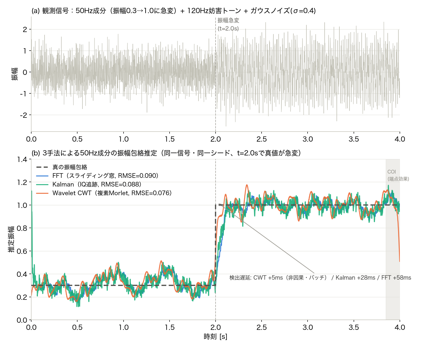
タスク設定:既知周波数成分の振幅急変をノイズの中から追跡する
設定は軸受欠陥の特徴周波数 50Hz が、ある時刻から急に強くなる状況を模したものである。50Hz 成分に 120Hz の妨害トーン( FFT 記事 と同じ周波数)とガウスノイズを重ね、\(t=2.0\) s で振幅が 0.3 → 1.0 へ階段状に変化する。
import numpy as np
from scipy.signal import stft
import pywt
import time

np.random.seed(0)
fs = 1000.0          # サンプリング周波数 [Hz]
T = 4.0              # 信号長 [s]
N = int(fs * T)
t = np.arange(N) / fs
f0 = 50.0            # 追跡対象の既知周波数(軸受欠陥の特徴周波数を想定)
f_interferer = 120.0 # 妨害トーン

A_true = np.where(t < 2.0, 0.3, 1.0)  # 真の振幅包絡:t=2.0sで階段状に急変
x_clean = A_true * np.sin(2 * np.pi * f0 * t) + 0.5 * np.sin(2 * np.pi * f_interferer * t)
noise_sigma = 0.4
x = x_clean + noise_sigma * np.random.randn(N)
w0 = 2 * np.pi * f0 / fs
3 手法すべてに「時刻 \(t\) における 50Hz 成分の振幅を推定せよ」という同一タスクを課す。
手法1: FFT(スライディング窓による単一ビン抽出、因果的)
窓長 \(L=100\) サンプル(100ms = 5 周期)で、\(f_s/L=10\) Hz ごとのビンに 50Hz・120Hz がちょうど乗るため、矩形窓のままリーク無く抽出できる。
L = 100
cos_ref = np.cos(w0 * np.arange(L))
sin_ref = np.sin(w0 * np.arange(L))
amp_fft = np.full(N, np.nan)
for n in range(L, N + 1):
    seg = x[n - L:n]
    c, s = seg @ cos_ref, seg @ sin_ref
    amp_fft[n - 1] = (2.0 / L) * np.sqrt(c ** 2 + s ** 2)
手法2: Kalman フィルタ(単一周波数 IQ 追跡、逐次・因果的)
https://yuhi-sa.github.io/posts/20260224_kalman_filter/1/の状態ベクトルは位置・速度 \([p, v]^T\) だったが、ここでは振幅追跡用の状態モデルとして、既知の角周波数 \(\omega_0\) で回転する IQ 成分 \([a_k, b_k]^T\) を状態に取る。観測モデルは時刻ごとに基準波形 \(\cos(\omega_0 k), \sin(\omega_0 k)\) で内積を取る形になる:
\[ y_k = a_k \cos(\omega_0 k) + b_k \sin(\omega_0 k) + v_k \]\(a_k, b_k\) をランダムウォーク(過程ノイズ \(Q\) )でゆっくり変化させることで、振幅の急変にも追従できる。振幅推定値は \(\sqrt{a_k^2 + b_k^2}\) 。
def run_kalman(x, w0, q, r):
    n = len(x)
    xk, P = np.zeros(2), np.eye(2)
    Q, amp = np.eye(2) * q, np.zeros(n)
    for k in range(n):
        P = P + Q  # 予測(ランダムウォーク)
        H = np.array([np.cos(w0 * k), np.sin(w0 * k)])
        y_pred = H @ xk
        S = H @ P @ H.T + r
        K = (P @ H) / S
        xk = xk + K * (x[k] - y_pred)
        P = P - np.outer(K, H @ P)
        amp[k] = np.sqrt(xk[0] ** 2 + xk[1] ** 2)
    return amp

# Qをグリッドサーチ(過渡追従と定常ノイズ耐性のトレードオフ)
r_meas = noise_sigma ** 2 + 0.5 * 0.5 ** 2  # 妨害トーンの寄与を観測ノイズとして概算
best_q = min([1e-6, 1e-5, 3e-5, 1e-4, 3e-4, 1e-3, 1e-2],
             key=lambda q: np.sqrt(np.mean((run_kalman(x, w0, q, r_meas)[100:] - A_true[100:]) ** 2)))
amp_kalman = run_kalman(x, w0, best_q, r_meas)
グリッドサーチの結果 \(Q=3\times10^{-4}\) が RMSE 最小だった。
手法3: Wavelet CWT(複素 Morlet、バッチ処理・非因果的)
https://yuhi-sa.github.io/posts/20260226_wavelet/1/やhttps://yuhi-sa.github.io/posts/20260524_time_frequency_guide/1/の実測コードは実数値 "morl" を使っていたが、これは瞬時周波数のリッジ追跡には十分でも、振幅包絡の抽出には不向きである(実数ウェーブレットとの畳み込みは搬送波の周期で振動するため)。
Hilbert 変換
の解析信号と同じ発想で、複素 Morlet "cmor1.5-1.0" を使い、係数の絶対値を包絡として使う。
wavelet_name = "cmor1.5-1.0"
scale_f0 = pywt.frequency2scale(wavelet_name, f0 / fs)
coef, freqs_cwt = pywt.cwt(x, [scale_f0], wavelet_name, sampling_period=1 / fs)
amp_cwt_raw = np.abs(coef[0])

# CWT係数の絶対値は物理振幅と直接一致しないため定常区間(t=3.0-3.8s, 真値1.0)で校正
# 3.8-4.0sは端点効果(cone of influence)がかかるため校正区間から除外
calib_mask = (t >= 3.0) & (t <= 3.8)
calib_factor = 1.0 / np.mean(amp_cwt_raw[calib_mask])
amp_cwt = amp_cwt_raw * calib_factor
出力:
CWT scale for 50.0Hz: 20.000, calibration factor: 0.4551
比較結果:精度・頑健性・計算コスト
末尾 0.15s(CWT の端点効果区間)と先頭 0.1s(FFT のウォームアップ区間)を全手法共通で除外し、RMSE・定常区間の標準偏差・検出遅延(閾値 0.65 を最初に超える時刻と真の変化時刻 \(t=2.0\) s との差)・実行時間(5 回平均)を実測した。
| 手法 | RMSE | 定常偏差(急変前) | 定常偏差(急変後) | 検出遅延 | 実行時間(5回平均) |
|---|---|---|---|---|---|
| FFT(スライディング窓) | 0.090 | 0.070 | 0.044 | +58ms | 5.83ms |
| Kalman(IQ追跡) | 0.088 | 0.073 | 0.054 | +28ms | 26.94ms |
| Wavelet CWT(複素Morlet) | 0.076 | 0.079 | 0.061 | +5ms | 0.70ms |
3 手法とも RMSE は 0.08 前後で拮抗しているが、検出遅延と実行時間には大きな差が出た。CWT は真の変化から 5ms 以内に検出できているが、これは全信号を一度に処理するバッチ処理(非因果的)だからである。中心対称なウェーブレットで畳み込むため、変化点の前後の情報を両方使って推定でき、見かけ上ほぼ即座に検出できる。対照的に、Kalman と FFT は時刻 \(k\)
までの観測しか使わない因果的な推定であり、原理的に遅延なしでは検出できない。CWT の実行時間が最速なのは、単一スケールへの畳み込みが pywt.cwt 内部でベクトル化されているのに対し、上記の FFT・Kalman 実装は Python ループのままだからでもある(実運用では FFT ベースの畳み込みで高速化できる)。
下図はこの3手法の推定結果を1つの図に重ねたものである。
ノイズレベル別のロバスト性:手法間で優劣が入れ替わる
ノイズ標準偏差 \(\sigma\) を 0.2/0.4/0.8/1.2 と変えて同じ実験を繰り返すと、低ノイズ帯と高ノイズ帯で最良手法が入れ替わるという興味深い結果が得られた。
| \(\sigma\) | FFT | Kalman | Wavelet CWT |
|---|---|---|---|
| 0.2 | 0.073 | 0.067 | 0.043 |
| 0.4 | 0.090 | 0.088 | 0.076 |
| 0.8 | 0.132 | 0.126 | 0.141 |
| 1.2 | 0.176 | 0.157 | 0.203 |
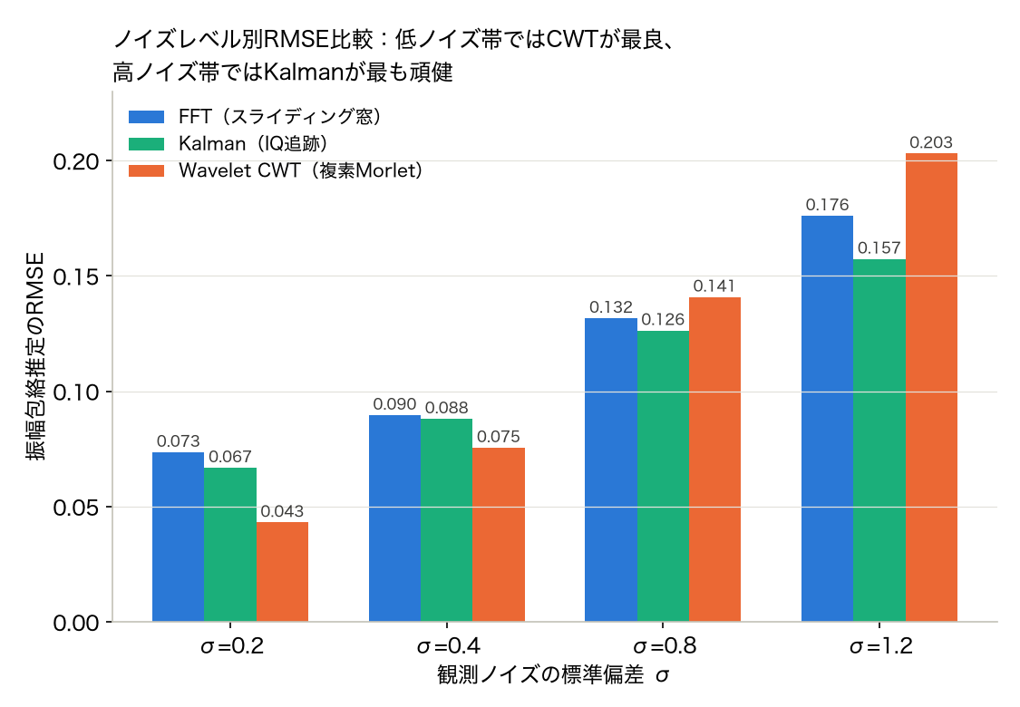
低ノイズ帯(\(\sigma \le 0.4\) )では CWT が最も高精度だが、高ノイズ帯(\(\sigma \ge 0.8\) )では Kalman フィルタが最も頑健になり、CWT は逆に最下位に転落する。これは、CWT の校正係数が固定(定常区間での 1 点校正)であるのに対し、Kalman フィルタは観測ノイズ共分散 \(R\) を通じてノイズレベルに応じたゲイン調整を明示的に行う最適推定だからである。「ノイズレベルが未知・変動する」現場では Kalman の適応性が効いてくる。
Kalman の過程ノイズ \(Q\) 感度:応答性とノイズ耐性のトレードオフ実測
Kalman フィルタの過程ノイズ \(Q\) は「振幅の急変にどれだけ素早く追従するか」と「定常時にどれだけノイズに惑わされないか」のトレードオフを直接制御する。実測すると:
| \(Q\) 設定 | RMSE | 検出遅延 |
|---|---|---|
| 過小 (\(10^{-6}\) ) | 0.224 | +527ms |
| 最適 (\(3\times10^{-4}\) ) | 0.088 | +28ms |
| 過大 (\(10^{-2}\) ) | 0.178 | 負(誤警報) |
\(Q\) が過小だと状態がほぼ固定され、急変への追従に 527ms もかかる。\(Q\) が過大だと逆にノイズに敏感になりすぎ、真の変化点(\(t=2.0\) s)より前に閾値を超えてしまう(見かけ上「負の遅延」)。ただしこれは CWT のような非因果的な早期検出とは異なり、ノイズによる誤警報である。Kalman は因果的な手法なので未来の情報を使えず、負の遅延が出るのは必ず「早すぎる誤検出」であって「正しい早期検出」ではない。この設定ではノイズだけで閾値を頻繁に超えるようになるため、「最初の閾値越え」の具体的なタイミング(負の遅延の絶対値)は誤警報が起き始める瞬間の定義に敏感で、実装の細部によって大きく変動しうる——ここでは符号(正しい方向より早いか遅いか)と誤警報である点にのみ着目し、絶対値は断定しない。実務で \(Q\) を選ぶ際は、\(Q\) のグリッドサーチだけでなく、閾値越えが真の変化点付近に集中しているか(誤警報率)も必ず確認する必要がある。
決定フレームワーク:実測結果に基づく手法選択
上記の実測から、以下の判断基準が導ける。
- バッチ処理が許され、ノイズレベルが低〜中程度で既知なら → Wavelet(複素 Morlet)。校正さえ済ませれば最高精度・最速の実行時間が得られる。ただし信号境界(cone of influence)の扱いに注意。
- リアルタイム・低遅延が必須(因果的な逐次処理が必要)なら → Kalman フィルタ。FFT より低遅延(本実験で 28ms vs 58ms)かつノイズレベル変動への適応性が高い。
- ノイズレベルが高い、または未知で変動するなら → Kalman フィルタ。観測ノイズ共分散 \(R\) を通じた最適ゲイン調整が、固定校正の CWT より頑健である。
- 実装の単純さ・検証のしやすさを優先するなら → FFT(スライディング窓)。パラメータは窓長 \(L\) のみで、周波数分解能 \(f_s/L\) から直感的に決められる。ただし検出遅延は 3 手法中最大になりやすい。
- リアルタイム性とノイズ頑健性の両方が必要なら → 本実験の Kalman がその中間解だが、\(Q\) のチューニングを誤ると「過小遅延・過大誤警報」のどちらかに転ぶ。前節のグリッドサーチと誤警報率の確認を必ず行う。
最新研究動向:Kalman フィルタの周波数選択性をニューラルネットで補強する
本実験で明らかになった Kalman フィルタの弱点は、周波数領域のノイズ構造(本実験では 120Hz の妨害トーン)を観測ノイズ \(R\) の中に一括して押し込めている点にある。この制約に正面から取り組む研究として、Dogan・Demirel・Holz が発表した FW-NKF(Frequency-Weighted Neural Kalman Filters) は、カルマンフィルタのイノベーション(観測残差)に因果的なスペクトル整形演算子を組み込み、観測モデルと遷移モデルをニューラルネットで学習することで、振動やバンド限定ノイズなど周波数依存の外乱を明示的に抑制する(Dogan, Demirel, Holz, FW-NKF: Frequency-Weighted Neural Kalman Filters, ICRA 2026, https://arxiv.org/abs/2606.02251 )。本実験で見た「Kalman は R に妨害トーンを丸めて詰め込んでいる」という単純化そのものを、学習可能なスペクトル演算子で置き換えようという発想であり、DSP の状態推定とニューラルネットの表現力を組み合わせる近年の潮流を象徴している。
7. 学習チェックリスト(40 項目)
数学基礎
- 複素指数関数 \(e^{j\omega t}\) の物理的意味が言える
- ラプラス変換と Fourier 変換の関係を説明できる
- 線形時不変システムの伝達関数を求められる
- Parseval の等式が書ける
- ナイキストの定理を説明できる
Bode / フィルタ設計
- 1 次ローパスのカットオフ周波数を \(-3\) dB から定義できる
- Butterworth と Chebyshev の通過域・阻止域特性を比較できる
- Bessel が群遅延平坦である理由を言える
scipy.signal.butterの出力をscipy.signal.lfilterに渡せる- IIR と FIR の安定性・線形位相特性を比較できる
- Notch フィルタの \(Q\) 値と帯域幅の関係を言える
- 双線形変換 z 変換の役割が説明できる
Fourier / 時間周波数
numpy.fft.fftの出力長と周波数軸を計算できる- 窓関数(Hann/Hamming/Blackman)のスペクトル漏れ抑制を比較できる
- PSD の単位(V²/Hz)を言える
- STFT のフレーム長 / ホップ長を信号特性から選べる
- CWT と DWT の違いを言える
- Wavelet Packet が CWT より高解像度な理由を言える
- Hilbert 変換と解析信号の関係を式で書ける
- EMD と VMD のモード混合の違いを言える
- SSA の窓長 \(L\) を周期から決められる
ML 時系列
- k-means の K を Elbow / Silhouette で決められる
- GMM の EM 更新式を書ける
- RandomForest と GBDT の違いを言える
- LSTM のゲート 3 種(input/forget/output)を説明できる
- IsolationForest の異常スコアの計算方法が言える
- 時系列の train/val/test 分割で leakage を避ける方法を知る
- Kalman フィルタの予測・更新式を書ける
- EKF と UKF のヤコビアン不要性の違いを言える
確率的最適化
- CEM の精英率(elite rate)の影響を言える
- SA の温度スケジュールを設計できる
- GA の交叉・突然変異の典型実装を書ける
- MPPI が CEM の重み付きサンプリングと類比できる
- ベイズ最適化の獲得関数(EI/PI/UCB)を比較できる
統合スキル
- センサデータ → フィルタ → 特徴量 → 分類のパイプラインを書ける
- STFT で前処理した特徴量を IsolationForest に渡せる
- SSA でトレンド除去後 LSTM 予測ができる
- ハイパーパラメータ最適化をベイズ最適化で実装できる
- matplotlib で複数サブプロットの可視化ができる
- 結果を再現可能にするため
numpy.random.seedを設定できる
8. よくある詰まりポイント Q&A
Q1. FFT の結果の周波数軸がわからない
np.fft.fftfreq(N, d=1/fs) または np.fft.rfftfreq(N, d=1/fs) で軸を生成する。サンプリング周波数 fs を必ず渡す。
Q2. フィルタが暴れる
scipy.signal.butter の正規化周波数は Nyquist=fs/2 で割った値。Wn=cutoff/(fs/2) を渡すか、scipy.signal.butter(..., fs=fs) の fs キーワードを使う。
Q3. LSTM の学習が進まない
入力スケーリング不足が最頻原因。sklearn.preprocessing.StandardScaler で平均 0 ・分散 1 にしてから学習。
Q4. STFT の窓長が選べない
周期最低 5〜10 周期入る長さに。nperseg = int(5 / target_freq * fs) を目安に試行錯誤。
Q5. EMD と VMD のどちらを使うか
モード数事前に決められる/安定性重視なら VMD、適応的に探索したいなら EMD(または EEMD)。詳細は https://yuhi-sa.github.io/posts/20260528_mode_decomposition/1/。
Q6. 異常検知で偽陽性が多い
特徴量に Hilbert 包絡線・Wavelet エネルギー・STFT バンド平均など信号の局所性を反映させる。IsolationForest の contamination パラメータの調整も有効。
Q7. ベイズ最適化の試行回数が足りない
低コスト目的関数では Grid Search が、高コストでは BO が有利。試行 50 回で頭打ちなら獲得関数を EI → UCB に切替。
9. 関連記事・参考資料
5 大ハブ:
- https://yuhi-sa.github.io/posts/20260521_bode_plot/1/ — Bode 線図ハブ
- https://yuhi-sa.github.io/posts/20260522_monte_carlo_optimization/1/ — モンテカルロ最適化ハブ
- https://yuhi-sa.github.io/posts/20260522_filter_design_guide/1/ — フィルタ設計指針ハブ
- https://yuhi-sa.github.io/posts/20260524_time_frequency_guide/1/ — 時間周波数解析ハブ
- https://yuhi-sa.github.io/posts/20260525_ml_timeseries_guide/1/ — 機械学習時系列ハブ
主要構成記事:
- https://yuhi-sa.github.io/posts/20260225_fft/1/ / https://yuhi-sa.github.io/posts/20260228_fft_window_psd/1/ / https://yuhi-sa.github.io/posts/20260429_stft/1/
- https://yuhi-sa.github.io/posts/20260226_wavelet/1/ / https://yuhi-sa.github.io/posts/20260522_wavelet_packet/1/ / https://yuhi-sa.github.io/posts/20260318_hilbert_transform/1/ / https://yuhi-sa.github.io/posts/20260528_mode_decomposition/1/
- https://yuhi-sa.github.io/posts/20260226_butterworth/1/ / https://yuhi-sa.github.io/posts/20260314_chebyshev_filter/1/ / https://yuhi-sa.github.io/posts/20260316_bessel_filter/1/ / https://yuhi-sa.github.io/posts/20260226_fir_iir/1/
- https://yuhi-sa.github.io/posts/20260228_notch_filter/1/ / https://yuhi-sa.github.io/posts/20260312_bandpass_filter/1/ / https://yuhi-sa.github.io/posts/20260313_highpass_filter/1/ / https://yuhi-sa.github.io/posts/20260223_lowpass_filter/1/
- https://yuhi-sa.github.io/posts/20260224_kalman_filter/1/ / https://yuhi-sa.github.io/posts/20260224_ekf/1/ / https://yuhi-sa.github.io/posts/20260226_ukf/1/ / https://yuhi-sa.github.io/posts/20260223_particle_filter/1/ / https://yuhi-sa.github.io/posts/20260223_rts_smoother/1/
- https://yuhi-sa.github.io/posts/20260226_kmeans_gmm/1/ / https://yuhi-sa.github.io/posts/20260226_ensemble_learning/1/ / https://yuhi-sa.github.io/posts/20260317_lstm_timeseries/1/ / https://yuhi-sa.github.io/posts/20260228_timeseries_anomaly/1/
- https://yuhi-sa.github.io/posts/20260223_bayesian_optimization/1/ / https://yuhi-sa.github.io/posts/20210329_cem/1/ / https://yuhi-sa.github.io/posts/20260226_simulated_annealing/1/ / https://yuhi-sa.github.io/posts/20260226_genetic_algorithm/1/ / https://yuhi-sa.github.io/posts/20260215_mppi/1/
第 9R で追加された新規ハブ・記事(5 大ハブ → 8 大ハブへの拡張)
過去サイクルで離散 DSP 基礎ハブ・モード分解ハブが追加され、本サイクル(第 10R)でさらに暗号系ハブが加わり、本ロードマップは 8 大ハブ体制 に拡張された。
- https://yuhi-sa.github.io/posts/20260613_discrete_dsp_basics/1/ — 離散 DSP 基礎ハブ(標本化定理 / DTFT・DFT・FFT / Z 変換 / 自己相関 / DCT)。本ロードマップの「DSP 入門」レイヤーの正式な入口。
- https://yuhi-sa.github.io/posts/20260528_mode_decomposition/1/ — モード分解ハブ(EMD / VMD / SSA)。非定常信号の前処理として ML 時系列ハブの上流に位置づく。
- https://yuhi-sa.github.io/posts/20260614_cryptography_roadmap/1/ — 暗号ロードマップハブ(対称鍵 / 公開鍵 / ハッシュ / 鍵交換)。DSP/ML とは別軸の「セキュリティ系」だが、繰り返し二乗法・離散数学が DSP の整数アルゴリズム群と接続する。
加えて ML 時系列ハブの 第 5 の柱 として Transformer 系時系列モデルを追加した:
- https://yuhi-sa.github.io/posts/20260614_transformer_timeseries/1/ — Transformer による時系列予測。LSTM の長期依存の限界を Self-Attention で克服し、Informer / Autoformer / TimesNet 系列を整理する。本ロードマップの「ML 時系列」レイヤーで LSTM の次のステップとして位置づく。
おすすめ書籍
サンプリング、FFT、フィルタ設計といったDSPの基礎理論をPythonコード付きで体系的に解説した一冊です。本ロードマップの各ハブ記事と合わせて読むことで、scipy.signal 中心の実装知識を理論面から補強できます。
※ 上記は Amazon アソシエイトのリンクです。
信号処理・機械学習・時系列・制御・暗号の各分野の書籍をレベル別にまとめた Pythonで信号処理・機械学習・制御を学ぶおすすめ技術書12選 も用意しています。本ロードマップと合わせて、自分のレベルに合った一冊を選ぶ参考にしてください。